Self-Supervised Learning: From Word Embeddings to Modern Vision-Language Models
Table of Contents
- Introduction
- Foundations of Self-Supervised Learning
- Evolution of Language Models
- Modality-Specific Self-Supervised Learning
- Multimodal Self-Supervised Learning
- Modern Vision-Language Models
- Training Strategies and Scaling Laws
- Current Challenges and Future Directions
- Practical Implementation Guide
- References
Introduction
Self-Supervised Learning (SSL) has revolutionized machine learning by eliminating the dependency on manually labeled datasets. Instead of requiring expensive human annotations, SSL methods create pretext tasks where the supervision signal emerges naturally from the data structure itself.
Core Principle
"Predict parts of the data from other parts of the data"
This fundamental insight, first formalized in Representation Learning: A Review and New Perspectives by Bengio et al. (2013), has enabled:
- Massive scalability with unlimited unlabeled data
- Rich representation learning that captures underlying data structures
- Transfer learning capabilities across diverse domains
- Foundation for modern AI including GPT, BERT, and Vision-Language Models
Why SSL Matters
Traditional supervised learning faces several limitations, as highlighted in Self-supervised Learning: Generative or Contrastive by Liu et al. (2021):
- Data bottleneck: Labeled datasets are expensive and time-consuming to create
- Domain specificity: Models trained on specific tasks don't generalize well
- Scalability issues: Human annotation doesn't scale with data growth
SSL addresses these by leveraging the inherent structure in data, making it possible to train on virtually unlimited amounts of unlabeled data from the internet, books, images, videos, and audio.
Theoretical Foundations: Why SSL Works
Core References: - A Simple Framework for Contrastive Learning of Visual Representations (SimCLR, Chen et al., 2020) - Momentum Contrast for Unsupervised Visual Representation Learning (MoCo, He et al., 2020) - Understanding Contrastive Representation Learning through Alignment and Uniformity (Wang & Isola, 2020)
Self-supervised pretraining works because it:
- Maximizes mutual information between different parts or views of the data (Understanding Contrastive Representation Learning).
- Injects useful inductive biases through the pretext task design (e.g., MLM in text, masked patches in vision).
- Exploits unlimited raw data to learn dense, transferable representations.
- Scales gracefully in both data and model size, following empirical scaling laws (Scaling Laws for Neural Language Models).
Mathematical Framework
From a representation-learning perspective, SSL encourages:
-
Invariance: Embeddings remain stable under transformations that should not affect meaning. [ f(T(x)) \approx f(x) ] Example: Random crop or color jitter in an image should not change the “cat-ness” of its representation.
-
Equivariance: Embeddings change in a predictable way under transformations that should affect meaning. [ f(T(x)) \approx T'(f(x)) ] Example: Translating an image left results in a proportionate shift in the feature map.
These invariances and equivariances are what make SSL embeddings transfer well: the model ignores irrelevant variation while consistently responding to meaningful changes, enabling strong performance on new tasks with minimal labeled data.
Key Papers on Invariance/Equivariance: - Invariant Risk Minimization (Arjovsky et al., 2019) - Group Equivariant Convolutional Networks (Cohen & Welling, 2016) - Data-Efficient Image Recognition with Contrastive Predictive Coding (Hénaff et al., 2019)
Training Dynamics: Underfitting vs. Overfitting in SSL
Key References: - Exploring the Limits of Weakly Supervised Pretraining (Mahajan et al., 2018) - Rethinking ImageNet Pre-training (He et al., 2018) - A Large-scale Study of Representation Learning with the Visual Task Adaptation Benchmark (Zhai et al., 2019)
In large-scale SSL pretraining, mild underfitting is the norm:
- Underfitting is common because:
- The datasets are enormous (often billions of examples).
- Pretext tasks (masking, contrastive alignment) are intentionally challenging.
- The goal is not to perfectly solve the pretext task, but to learn generalizable features.
-
Example: In BERT's MLM (BERT: Pre-training of Deep Bidirectional Transformers), final pretraining accuracy on masked tokens often stays in the 40–70% range.
-
Overfitting can happen when:
- The dataset is small or lacks diversity.
- The pretext task is too easy (low-entropy target space).
- Training runs for too long without data refresh or augmentation.
- Symptoms: Pretext loss keeps dropping but downstream task performance stagnates or drops.
Good practice (A Large-scale Study of Representation Learning): - Monitor both pretext and downstream metrics. - Use large, diverse datasets and strong augmentations. - Stop training when downstream transfer stops improving. - Apply early stopping based on validation performance on downstream tasks.
| SSL stage | Common case | Why | Risk |
|---|---|---|---|
| Large-scale pretraining | Underfitting | Data >> model capacity; hard tasks | Slow convergence if model too small |
| Small-scale pretraining | Overfitting | Model memorizes dataset | Poor transferability |
| Fine-tuning on small labeled data | Overfitting | Labels are few | Needs strong regularization |
Cognitive Science Perspective: Human Analogy
Relevant Research: - The "Bootstrap" Approach to Language Learning (Pinker, 1999) - Predictive Processing: A Canonical Principle for Brain Function? (Keller & Mrsic-Flogel, 2018) - Self-supervised learning through the eyes of a child (Orhan et al., 2020)
Humans learn in a way that closely resembles mild underfitting in SSL:
- We don’t memorize everything: Our brains are exposed to massive, noisy sensory streams, but we store compressed, abstract representations (e.g., the concept of “tree” rather than the pixel values of every tree seen).
- We generate our own training signals: We predict words before they’re spoken, fill in missing letters in handwriting, and link sounds to objects — all without explicit labels.
- We underfit in a beneficial way:
- Capacity limits force us to filter out irrelevant details.
- Abstraction enables transfer to novel situations.
- Avoiding “perfect fit” prevents over-specialization to one environment.
Parallel to SSL:
| Aspect | Human learning | SSL |
|---|---|---|
| Data volume | Continuous, massive sensory input | Internet-scale unlabeled corpora |
| Objective | Predict/make sense of context | Pretext loss (masking, contrastive, etc.) |
| Fit level | Mild underfitting | Mild underfitting |
| Outcome | Broad, transferable knowledge | Broad, transferable features |
Key takeaway:
Just as humans don’t strive to perfectly predict every sensory input, SSL models benefit from leaving some pretext error on the table — it signals they’re capturing general patterns rather than memorizing specifics.
Foundations of Self-Supervised Learning
Information Theory Perspective
SSL can be understood through the lens of information theory. The goal is to learn representations that capture the most informative aspects of the data while discarding noise.
Mutual Information Maximization:
Where: - \(X\) represents the input data - \(Z\) represents the learned representation - \(I(X; Z)\) measures how much information \(Z\) contains about \(X\)
The Information Bottleneck Principle
SSL methods implicitly implement the Information Bottleneck principle:
This balances: - Compression: Minimize \(I(X; Z)\) to learn compact representations - Prediction: Maximize \(I(Z; Y)\) to retain task-relevant information
Pretext Task Design
Effective pretext tasks share common characteristics:
- Semantic preservation: The task should require understanding of meaningful content
- Scalability: Must work with unlimited unlabeled data
- Transferability: Learned representations should generalize to downstream tasks
Evolution of Language Models
Word2Vec: The Foundation
Historical Context: Before Word2Vec (Mikolov et al., 2013), word representations were primarily based on sparse count-based methods like Latent Semantic Analysis (LSA) or co-occurrence matrices.
Paper: Efficient Estimation of Word Representations in Vector Space
Code: Original C implementation | Gensim Python
Skip-gram Architecture
The Skip-gram model predicts context words given a target word:
Where: - \(T\) is the total number of words in the corpus - \(c\) is the context window size - \(w_t\) is the target word at position \(t\) - \(w_{t+j}\) are the context words
Negative Sampling Optimization
To make training computationally feasible, Word2Vec uses negative sampling:
Where: - \(\sigma\) is the sigmoid function - \(\mathbf{v}_{w_i}\) is the input vector for word \(w_i\) - \(\mathbf{v}'_{w_o}\) is the output vector for word \(w_o\) - \(K\) is the number of negative samples - \(P_n(w)\) is the noise distribution (typically \(P_n(w) \propto U(w)^{3/4}\))
Key Innovation: This approach transforms the multi-class classification problem into multiple binary classification problems, dramatically reducing computational complexity.
Impact and Legacy
- Dense representations: Moved from sparse 10,000+ dimensional vectors to dense 300-dimensional embeddings
- Semantic relationships: Captured analogies like "king - man + woman = queen"
- Foundation for contextualized embeddings: Inspired ELMo, GPT, and BERT
GPT: Autoregressive Language Modeling
Key Insight: Treat next-token prediction as a self-supervised task that can learn rich language representations.
Papers:
- GPT-1: Improving Language Understanding by Generative Pre-Training
- GPT-2: Language Models are Unsupervised Multitask Learners
- GPT-3: Language Models are Few-Shot Learners
Code: GPT-2 Official | Hugging Face Transformers
Causal Language Modeling Objective
Given a sequence of tokens \(w_1, w_2, ..., w_T\), GPT maximizes:
Where \(w_{<t} = w_1, w_2, ..., w_{t-1}\) represents all previous tokens.
Architecture Deep Dive
Transformer Decoder Stack: - Multi-head self-attention with causal masking - Position embeddings to encode sequence order - Layer normalization for training stability - Residual connections for gradient flow
Attention Mechanism:
With causal masking ensuring that position \(i\) can only attend to positions \(j \leq i\).
Scaling and Emergent Abilities
GPT Evolution: - GPT-1 (117M parameters): Demonstrated transfer learning potential - GPT-2 (1.5B parameters): Showed zero-shot task performance - GPT-3 (175B parameters): Exhibited few-shot learning and emergent abilities - GPT-4 (estimated 1.7T parameters): Multimodal capabilities and advanced reasoning
Emergent Abilities: As model size increases, new capabilities emerge that weren't explicitly trained for: - In-context learning - Chain-of-thought reasoning - Code generation - Mathematical problem solving
BERT: Bidirectional Contextualized Representations
Innovation: Unlike GPT's unidirectional approach, BERT uses bidirectional context to create richer representations.
Paper: BERT: Pre-training of Deep Bidirectional Transformers for Language Understanding
Code: Google Research BERT | Hugging Face

Masked Language Modeling (MLM)
BERT randomly masks 15% of input tokens and predicts them using bidirectional context:
Where: - \(\mathcal{M}\) is the set of masked positions - \(\mathbf{w}_{\setminus i}\) represents all tokens except the masked one
Masking Strategy: - 80% of the time: Replace with [MASK] token - 10% of the time: Replace with random token - 10% of the time: Keep original token
This prevents the model from simply copying the input during fine-tuning.
Next Sentence Prediction (NSP)
BERT also learns sentence-level relationships:
This helps the model understand document-level structure and relationships between sentences.
Advantages and Limitations
Advantages: - Full context: Uses both left and right context for each token - Strong performance: Achieved state-of-the-art on GLUE, SQuAD, and other benchmarks - Interpretability: Attention patterns often align with linguistic structures
Limitations: - Pretrain-finetune mismatch: [MASK] tokens not present during inference - Computational cost: Bidirectional attention is more expensive than causal - Generation limitations: Not naturally suited for text generation tasks
Modern Unified Approaches
T5: Text-to-Text Transfer Transformer
Philosophy: "Every NLP task can be framed as text-to-text"
Paper: Exploring the Limits of Transfer Learning with a Unified Text-to-Text Transformer
Code: Google Research T5 | Hugging Face T5
Span Corruption Objective:
T5 masks contiguous spans and trains the model to generate the missing text, combining the benefits of MLM and autoregressive generation.
Instruction Tuning and Alignment
InstructGPT/ChatGPT Pipeline: 1. Supervised Fine-tuning (SFT): Train on high-quality instruction-response pairs 2. Reward Modeling: Train a reward model to score responses 3. Reinforcement Learning from Human Feedback (RLHF): Optimize policy using PPO
RLHF Objective:
Where: - \(r_\phi(x, y)\) is the reward model score - \(\beta\) controls the KL penalty to prevent deviation from the reference model - \(\pi_{\text{ref}}\) is the SFT model used as reference
Modality-Specific Self-Supervised Learning
Audio: Wav2Vec and Beyond
Wav2Vec 2.0 Architecture
Paper: wav2vec 2.0: A Framework for Self-Supervised Learning of Speech Representations
Code: Facebook Research | Hugging Face
Pipeline: 1. Feature Encoder: Convolutional layers process raw waveform 2. Quantization: Vector quantization creates discrete targets 3. Masking: Random spans in latent space are masked 4. Context Network: Transformer processes masked sequence 5. Contrastive Learning: Predict correct quantized representation
Detailed Process:
Step 1 - Feature Encoding: \(\(\mathbf{z}_t = f_{\text{enc}}(\mathbf{x}_{t:t+\Delta})\)\)
Where \(f_{\text{enc}}\) is a 7-layer CNN that processes 25ms windows with 20ms stride.
Step 2 - Quantization: \(\(\mathbf{q}_t = \text{Quantize}(\mathbf{z}_t)\)\)
Using Gumbel-Softmax for differentiable quantization: \(\(\mathbf{q} = \sum_{j=1}^{V} \frac{\exp((\log \pi_j + g_j)/\tau)}{\sum_{k=1}^{V} \exp((\log \pi_k + g_k)/\tau)} \mathbf{e}_j\)\)
Step 3 - Contrastive Loss: \(\(\mathcal{L}_{\text{contrast}} = -\log \frac{\exp(\text{sim}(\mathbf{c}_t, \mathbf{q}_t) / \kappa)}{\sum_{\tilde{\mathbf{q}} \in \mathcal{Q}_t} \exp(\text{sim}(\mathbf{c}_t, \tilde{\mathbf{q}}) / \kappa)}\)\)
Where: - \(\mathbf{c}_t\) is the context vector from the Transformer - \(\mathbf{q}_t\) is the true quantized target - \(\mathcal{Q}_t\) includes \(\mathbf{q}_t\) plus \(K\) distractors - \(\kappa\) is the temperature parameter
Why This Works: - Temporal structure: Audio has rich temporal dependencies - Hierarchical features: From phonemes to words to sentences - Invariance learning: Model learns to ignore speaker-specific variations
HuBERT: Iterative Pseudo-labeling
Innovation: Instead of using quantization, HuBERT uses iterative clustering.
Paper: HuBERT: Self-Supervised Speech Representation Learning by Masked Prediction of Hidden Units
Code: Facebook Research | Hugging Face
Algorithm: 1. Initialize: Cluster MFCC features using k-means 2. Train: Predict cluster assignments with masked prediction 3. Re-cluster: Use learned representations for new clustering 4. Iterate: Repeat until convergence
Objective: \(\(\mathcal{L}_{\text{HuBERT}} = \sum_{t \in \mathcal{M}} \text{CrossEntropy}(f(\mathbf{h}_t), z_t)\)\)
Where \(z_t\) is the cluster assignment and \(\mathbf{h}_t\) is the contextualized representation.
Vision: From Contrastive to Generative
Contrastive Learning (SimCLR, MoCo)
Core Idea: Learn representations by contrasting positive and negative pairs.
Papers:
- SimCLR: A Simple Framework for Contrastive Learning of Visual Representations
- MoCo: Momentum Contrast for Unsupervised Visual Representation Learning
Code: SimCLR Official | MoCo Official

SimCLR Pipeline: 1. Augmentation: Apply two random augmentations to each image 2. Encoding: Pass through CNN encoder (e.g., ResNet) 3. Projection: Map to lower-dimensional space with MLP 4. Contrastive Loss: Maximize agreement between positive pairs
NT-Xent Loss: \(\(\mathcal{L}_{i,j} = -\log \frac{\exp(\text{sim}(\mathbf{z}_i, \mathbf{z}_j) / \tau)}{\sum_{k=1}^{2N} \mathbf{1}_{[k \neq i]} \exp(\text{sim}(\mathbf{z}_i, \mathbf{z}_k) / \tau)}\)\)
Where: - \((i, j)\) form a positive pair - \(\tau\) is the temperature parameter - \(N\) is the batch size (so \(2N\) total augmented samples)
Key Insights: - Large batch sizes are crucial (SimCLR uses 4096) - Strong augmentations force the model to learn invariant features - Projection head improves representation quality but is discarded after training
MoCo Innovation: Uses a momentum-updated encoder to maintain a large, consistent set of negative samples:
Where \(m \in [0, 1)\) is the momentum coefficient.
Masked Autoencoders (MAE)
Philosophy: "What I cannot create, I do not understand" - Richard Feynman
Paper: Masked Autoencoders Are Scalable Vision Learners
Code: Facebook Research | Hugging Face
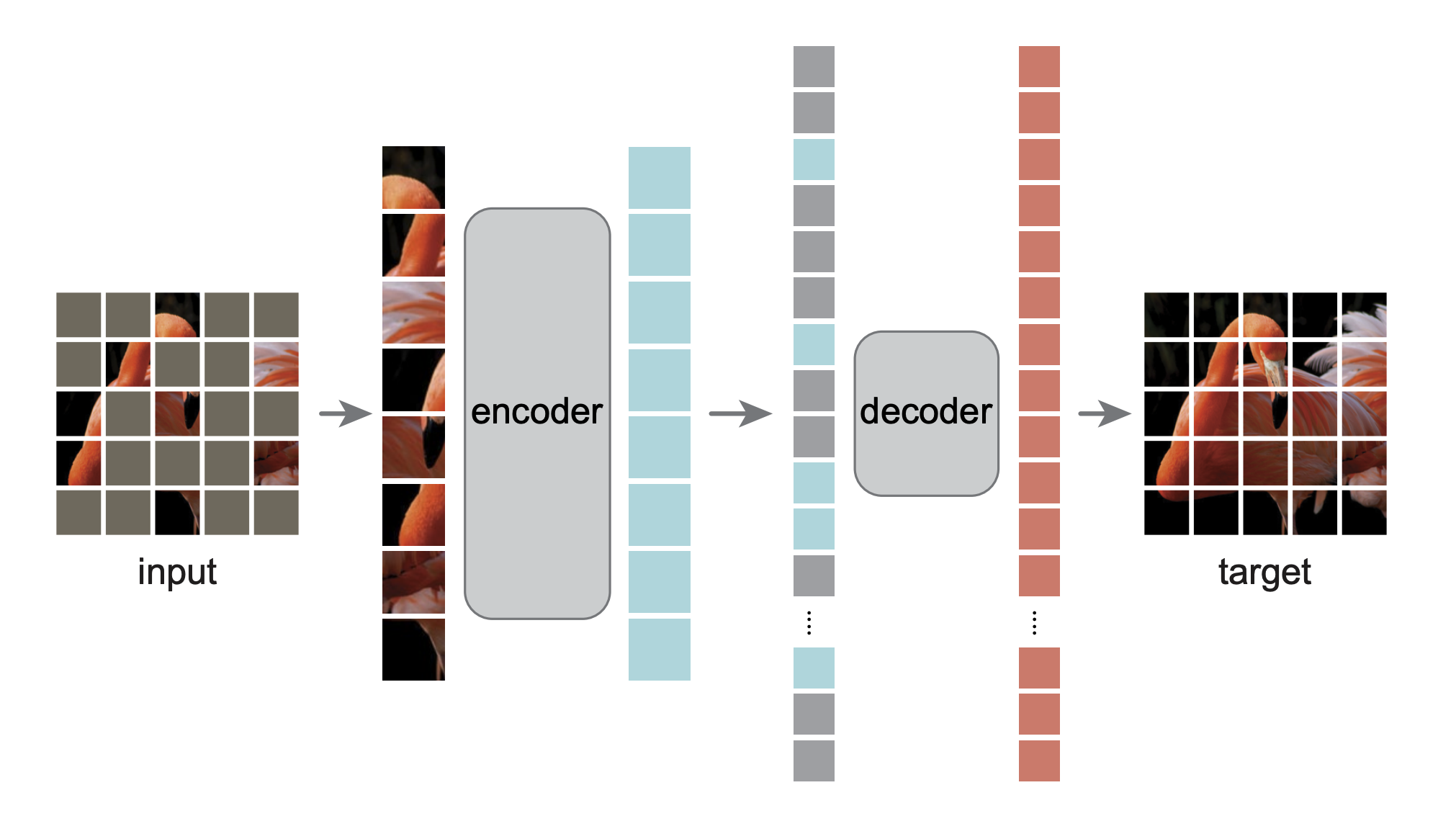
Architecture: 1. Patch Embedding: Divide image into 16×16 patches 2. Random Masking: Remove 75% of patches 3. Encoder: Process only visible patches with Vision Transformer 4. Decoder: Reconstruct masked patches from encoded representation
Objective: \(\(\mathcal{L}_{\text{MAE}} = \frac{1}{|\mathcal{M}|} \sum_{i \in \mathcal{M}} ||\mathbf{x}_i - \hat{\mathbf{x}}_i||_2^2\)\)
Where \(\mathcal{M}\) is the set of masked patches.
Why High Masking Ratio Works: - Forces global understanding: Can't rely on local texture patterns - Computational efficiency: Only process 25% of patches in encoder - Rich reconstruction task: Requires understanding of object structure and context
Comparison with NLP: - Information density: Images have higher spatial redundancy than text - Reconstruction target: Pixels vs. semantic tokens - Masking strategy: Random vs. structured (spans)
Multimodal Self-Supervised Learning
CLIP: Contrastive Language-Image Pre-training
Revolutionary Insight: Learn visual concepts from natural language supervision at scale.
Paper: Learning Transferable Visual Models From Natural Language Supervision
Code: OpenAI CLIP | Hugging Face

Architecture and Training
Dual Encoder Design: - Image Encoder: Vision Transformer or ResNet - Text Encoder: Transformer (similar to GPT-2) - Shared Embedding Space: Both modalities project to same dimensionality
Contrastive Objective (InfoNCE Loss): \(\(\mathcal{L}_{\text{CLIP}} = \frac{1}{2}(\mathcal{L}_{I \to T} + \mathcal{L}_{T \to I})\)\)
Where: \(\(\mathcal{L}_{I \to T} = -\frac{1}{N} \sum_{i=1}^N \log \frac{\exp(\mathbf{I}_i \cdot \mathbf{T}_i / \tau)}{\sum_{j=1}^N \exp(\mathbf{I}_i \cdot \mathbf{T}_j / \tau)}\)\)
Loss Function Details: - Name: InfoNCE (Information Noise Contrastive Estimation) - Symmetric: Both image-to-text and text-to-image directions - Temperature scaling: \(\tau\) controls the sharpness of the distribution - Batch-wise contrastive: Each sample contrasts against all others in the batch
Training Details: - Dataset: 400M image-text pairs from the internet - Batch size: 32,768 pairs - Temperature: \(\tau = 0.07\) - Optimization: AdamW with cosine learning rate schedule
Contrastive Learning Deep Dive
Core Principle: Learn representations by maximizing agreement between positive pairs while minimizing agreement with negative pairs.
Dataset Requirements: 1. Paired data: Each image must have corresponding text description 2. Diversity: Wide variety of concepts, objects, scenes, and descriptions 3. Scale: Large datasets (100M+ pairs) crucial for good performance 4. Quality vs. Quantity: CLIP shows that scale can overcome noise in web data 5. Natural language: Captions should be natural, descriptive text (not just labels)
Hard Negatives: - Definition: Negative samples that are semantically similar to positive samples - Examples: - Image of "dog" vs. text "cat" (both animals) - Image of "car" vs. text "truck" (both vehicles) - Importance: Force model to learn fine-grained distinctions - In CLIP: Naturally occur in large batches with diverse content - Mining strategies: Can be explicitly mined using similarity metrics
Batch Construction:
Batch of N image-text pairs:
- N positive pairs: (I₁,T₁), (I₂,T₂), ..., (Iₙ,Tₙ)
- N×(N-1) negative pairs: All cross-combinations
- Hard negatives emerge naturally from semantic diversity
Zero-Shot Transfer
Mechanism: Convert classification into image-text matching: 1. Template: "A photo of a {class}" 2. Encode: Get text embeddings for all class templates 3. Compare: Find closest text embedding to image embedding 4. Predict: Class with highest similarity
Mathematical Formulation: \(\(P(y = c | \mathbf{x}) = \frac{\exp(\text{sim}(f(\mathbf{x}), g(t_c)) / \tau)}{\sum_{i=1}^C \exp(\text{sim}(f(\mathbf{x}), g(t_i)) / \tau)}\)\)
Where: - \(f(\mathbf{x})\) is the image embedding - \(g(t_c)\) is the text embedding for class \(c\) - \(t_c\) is the text template for class \(c\)
Impact and Applications
Capabilities: - Zero-shot classification: Competitive with supervised models - Robustness: Better performance on distribution shifts - Flexibility: Easy to add new classes without retraining - Multimodal understanding: Bridges vision and language
Applications: - Image search: Natural language queries - Content moderation: Detect inappropriate content - Accessibility: Generate image descriptions - Creative tools: Text-to-image generation (DALL-E)
CLIP Extensions and Variants
GLIP: Grounded Language-Image Pre-training
Innovation: Unifies object detection and phrase grounding with CLIP-style training.
Paper: Grounded Language-Image Pre-training
Code: Microsoft GLIP
Key Features: - Grounded pre-training: Learn object-level vision-language alignment - Unified architecture: Single model for detection, grounding, and VQA - Rich annotations: Uses both detection and grounding datasets
Architecture:
Image → Vision Backbone → Region Features
Text → Language Encoder → Token Features
     ↓
Cross-modal Fusion → Detection Head
Training Objective: \(\(\mathcal{L}_{\text{GLIP}} = \mathcal{L}_{\text{detection}} + \mathcal{L}_{\text{grounding}} + \mathcal{L}_{\text{contrastive}}\)\)
GroundingDINO: Open-Set Object Detection
Philosophy: "Detect anything you can describe in natural language."
Paper: Grounding DINO: Marrying DINO with Grounded Pre-Training for Open-Set Object Detection
Code: IDEA Research
Key Innovations: - Transformer-based: DETR-style architecture with language conditioning - Open vocabulary: Can detect objects not seen during training - Phrase grounding: Localizes specific phrases in complex sentences
Architecture Components: 1. Feature Enhancer: Cross-modal feature fusion 2. Language-Guided Query Selection: Text-aware object queries 3. Cross-Modal Decoder: Joint vision-language reasoning
Training Strategy: - Multi-dataset training: Detection + grounding + caption datasets - Curriculum learning: From simple to complex grounding tasks - Pseudo-labeling: Generate labels for unlabeled detection data
OWL-ViT: Open-World Localization
Concept: "Vision Transformer for Open-World Localization"
Paper: Simple Open-Vocabulary Object Detection with Vision Transformers
Code: Google Research | Hugging Face
Architecture: - Base: Vision Transformer + Text Transformer (CLIP-style) - Detection head: Lightweight classification and box regression - Image patches: Each patch can be classified independently
Training Process: 1. CLIP pre-training: Learn general vision-language representations 2. Detection fine-tuning: Add detection head and train on detection data 3. Open-vocabulary inference: Use arbitrary text queries at test time
Mathematical Formulation: \(\(P(\text{class}|\text{patch}) = \text{softmax}(\text{sim}(f_{\text{patch}}, g_{\text{query}}) / \tau)\)\)
Comparison of CLIP Extensions
| Model | Strength | Use Case | Training Data |
|---|---|---|---|
| CLIP | General vision-language | Classification, retrieval | Image-text pairs |
| GLIP | Grounded understanding | Detection + grounding | Detection + grounding |
| GroundingDINO | Complex phrase grounding | Open-set detection | Multi-dataset fusion |
| OWL-ViT | Patch-level localization | Simple open detection | CLIP + detection data |
Recent Advances
CLIP-based Detection Models: - DetCLIP: Efficient open-vocabulary detection - RegionCLIP: Region-level CLIP training - GLIP-v2: Improved grounding with better data - FIBER: Fine-grained vision-language understanding
Key Trends: 1. Scaling: Larger models and datasets 2. Efficiency: Faster inference for real-time applications 3. Granularity: From image-level to pixel-level understanding 4. Multimodal reasoning: Beyond simple matching to complex reasoning
ALIGN: Scaling to Billion-Scale Data
Key Insight: Scale matters more than data quality for multimodal learning.
Paper: Scaling Up Visual and Vision-Language Representation Learning With Noisy Text Supervision
Code: Google Research
Differences from CLIP: - Dataset: 1.8B noisy image-text pairs (vs. CLIP's 400M curated) - Filtering: Minimal cleaning, embrace noise - Scale: Larger models and datasets
Results: Demonstrates that scale can overcome noise, achieving better performance than CLIP on many benchmarks.
Training Strategies and Scaling Laws
Data Scaling
Key Papers:
- Scaling Laws for Neural Language Models
- Training Compute-Optimal Large Language Models (Chinchilla)
- Scaling Laws for Autoregressive Generative Modeling
Compute Scaling
Chinchilla Scaling Laws: Optimal compute allocation between model size and training data.
Paper: Training Compute-Optimal Large Language Models
Key Finding: For a given compute budget, training smaller models on more data is often better than training larger models on less data.
Scaling Laws for Multimodal Models
Extension of Language Model Scaling:
For multimodal models, performance scales with:
Where: - \(N_v, N_l\): Vision and language model parameters - \(D_v, D_l\): Vision and language dataset sizes - \(C\): Compute budget - \(\alpha, \beta, \gamma\): Scaling exponents
Data Efficiency and Transfer Learning
Pre-training → Fine-tuning Paradigm:
- Large-scale pre-training: Learn general representations
- Task-specific fine-tuning: Adapt to downstream tasks
- Few-shot adaptation: Leverage in-context learning
Transfer Learning Effectiveness:
Empirical Observations: - More pre-training data → Better downstream performance - Larger models → Better few-shot learning - Diverse pre-training → Better generalization
Curriculum Learning and Progressive Training
Curriculum Design: 1. Easy examples first: Start with high-quality, clear examples 2. Gradual complexity: Increase task difficulty over time 3. Multi-task mixing: Balance different objectives
Example Curriculum for VLM:
Phase 1: High-quality image-caption pairs (COCO, Flickr30k)
Phase 2: Web-scraped image-text pairs (CC12M, LAION)
Phase 3: Complex reasoning tasks (VQA, visual reasoning)
Phase 4: Instruction following (LLaVA-style data)
Current Challenges and Future Directions
Efficiency and Sustainability
Relevant Papers:
- Green AI
- Energy and Policy Considerations for Deep Learning in NLP
- Carbon Emissions and Large Neural Network Training
Multimodal Reasoning
Key Papers:
- Multimodal Deep Learning for Robust RGB-D Object Recognition
- ViLBERT: Pretraining Task-Agnostic Visiolinguistic Representations for Vision-and-Language Tasks
- LXMERT: Learning Cross-Modality Encoder Representations from Transformers
Technical Challenges
1. Multimodal Alignment Drift
Problem: As models scale, maintaining alignment between modalities becomes challenging.
Solutions: - Regular alignment checks: Monitor cross-modal similarity during training - Balanced sampling: Ensure equal representation of modalities - Contrastive regularization: Add alignment losses throughout training
2. Computational Efficiency
Challenges: - Memory requirements: Large models need significant GPU memory - Training time: Multimodal models take longer to train - Inference cost: Real-time applications need efficient models
Solutions: - Model compression: Pruning, quantization, distillation - Efficient architectures: MobileViT, EfficientNet variants - Progressive training: Start small, gradually increase model size
3. Data Quality and Bias
Issues: - Web data noise: Internet data contains errors and biases - Representation bias: Underrepresentation of certain groups - Cultural bias: Models may not work well across cultures
Mitigation Strategies: - Careful curation: Filter and clean training data - Diverse datasets: Include data from multiple sources and cultures - Bias evaluation: Regular testing on diverse benchmarks - Fairness constraints: Add fairness objectives to training
Emerging Directions
1. Video Understanding
Challenges: - Temporal modeling: Understanding motion and temporal relationships - Long sequences: Processing hours of video content - Multi-granular understanding: From frames to scenes to stories
Approaches: - Video Transformers: Extend ViT to temporal dimension - Hierarchical processing: Different models for different time scales - Memory mechanisms: Store and retrieve relevant information
2. 3D and Spatial Understanding
Applications: - Robotics: Spatial reasoning for manipulation - Autonomous driving: 3D scene understanding - AR/VR: Spatial computing applications
Techniques: - 3D representations: Point clouds, meshes, neural radiance fields - Multi-view learning: Learn from multiple camera angles - Depth estimation: Infer 3D structure from 2D images
3. Embodied AI
Goal: Agents that can perceive, reason, and act in physical environments.
Components: - Perception: Multimodal understanding of environment - Planning: Long-term goal-oriented behavior - Control: Low-level motor skills and manipulation - Learning: Adaptation to new environments and tasks
Training Paradigms: - Simulation: Train in virtual environments (Isaac Gym, Habitat) - Real-world data: Collect interaction data from robots - Transfer learning: Sim-to-real domain adaptation
Practical Implementation Guide
Getting Started with CLIP
Installation and Setup:
pip install torch torchvision
pip install git+https://github.com/openai/CLIP.git
# or
pip install transformers
Hugging Face Integration:
from transformers import CLIPProcessor, CLIPModel

model = CLIPModel.from_pretrained("openai/clip-vit-base-patch32")
processor = CLIPProcessor.from_pretrained("openai/clip-vit-base-patch32")
Training Your Own Models
Useful Resources:
- OpenCLIP: Open source implementation of CLIP
- LAION Datasets - Large-scale image-text datasets
- Conceptual Captions - Google's image-text dataset
Evaluation and Benchmarks
Benchmark Papers and Datasets:
- GLUE: A Multi-Task Benchmark and Analysis Platform for Natural Language Understanding
- SuperGLUE: A Stickier Benchmark for General-Purpose Language Understanding Systems
- VQA: Visual Question Answering | Dataset
- COCO Captions | Dataset
- Flickr30K | Dataset
Setting Up a Multimodal Training Pipeline
1. Data Preparation
Dataset Collection:
# Example: Preparing image-text pairs
import torch
from torch.utils.data import Dataset, DataLoader
from PIL import Image
import json

class ImageTextDataset(Dataset):
    def __init__(self, data_path, transform=None):
        with open(data_path, 'r') as f:
            self.data = json.load(f)
        self.transform = transform

    def __len__(self):
        return len(self.data)

    def __getitem__(self, idx):
        item = self.data[idx]
        image = Image.open(item['image_path']).convert('RGB')
        text = item['caption']

        if self.transform:
            image = self.transform(image)

        return {
            'image': image,
            'text': text,
            'image_id': item.get('image_id', idx)
        }
Data Augmentation:
from torchvision import transforms

# Vision augmentations
vision_transform = transforms.Compose([
    transforms.RandomResizedCrop(224, scale=(0.8, 1.0)),
    transforms.RandomHorizontalFlip(p=0.5),
    transforms.ColorJitter(brightness=0.2, contrast=0.2, saturation=0.2),
    transforms.ToTensor(),
    transforms.Normalize(mean=[0.485, 0.456, 0.406],
                        std=[0.229, 0.224, 0.225])
])

# Text augmentations (example)
def augment_text(text):
    # Synonym replacement, back-translation, etc.
    return text
2. Model Architecture
Simple CLIP-style Model:
import torch
import torch.nn as nn
from transformers import CLIPVisionModel, CLIPTextModel

class SimpleVLM(nn.Module):
    def __init__(self, vision_model_name, text_model_name, embed_dim=512):
        super().__init__()

        # Vision encoder
        self.vision_encoder = CLIPVisionModel.from_pretrained(vision_model_name)
        self.vision_projection = nn.Linear(
            self.vision_encoder.config.hidden_size, embed_dim
        )

        # Text encoder
        self.text_encoder = CLIPTextModel.from_pretrained(text_model_name)
        self.text_projection = nn.Linear(
            self.text_encoder.config.hidden_size, embed_dim
        )

        # Temperature parameter
        self.temperature = nn.Parameter(torch.ones([]) * 0.07)

    def encode_image(self, images):
        vision_outputs = self.vision_encoder(images)
        image_embeds = self.vision_projection(vision_outputs.pooler_output)
        return F.normalize(image_embeds, dim=-1)

    def encode_text(self, input_ids, attention_mask):
        text_outputs = self.text_encoder(input_ids, attention_mask)
        text_embeds = self.text_projection(text_outputs.pooler_output)
        return F.normalize(text_embeds, dim=-1)

    def forward(self, images, input_ids, attention_mask):
        image_embeds = self.encode_image(images)
        text_embeds = self.encode_text(input_ids, attention_mask)

        # Contrastive loss
        logits_per_image = torch.matmul(image_embeds, text_embeds.t()) / self.temperature
        logits_per_text = logits_per_image.t()

        return logits_per_image, logits_per_text
3. Training Loop
Contrastive Training:
def train_epoch(model, dataloader, optimizer, device):
    model.train()
    total_loss = 0

    for batch in dataloader:
        images = batch['image'].to(device)
        input_ids = batch['input_ids'].to(device)
        attention_mask = batch['attention_mask'].to(device)

        optimizer.zero_grad()

        logits_per_image, logits_per_text = model(images, input_ids, attention_mask)

        # Symmetric cross-entropy loss
        batch_size = images.size(0)
        labels = torch.arange(batch_size).to(device)

        loss_img = F.cross_entropy(logits_per_image, labels)
        loss_txt = F.cross_entropy(logits_per_text, labels)
        loss = (loss_img + loss_txt) / 2

        loss.backward()
        optimizer.step()

        total_loss += loss.item()

    return total_loss / len(dataloader)
4. Evaluation and Metrics
Zero-shot Classification:
def zero_shot_classification(model, images, class_names, templates, device):
    model.eval()

    # Encode images
    with torch.no_grad():
        image_features = model.encode_image(images)

    # Encode class names with templates
    text_features = []
    for class_name in class_names:
        texts = [template.format(class_name) for template in templates]
        text_inputs = tokenizer(texts, padding=True, return_tensors='pt').to(device)

        with torch.no_grad():
            class_embeddings = model.encode_text(text_inputs['input_ids'],
                                                text_inputs['attention_mask'])
            class_embeddings = class_embeddings.mean(dim=0)  # Average over templates
            text_features.append(class_embeddings)

    text_features = torch.stack(text_features)

    # Compute similarities
    similarities = torch.matmul(image_features, text_features.t())
    predictions = similarities.argmax(dim=-1)

    return predictions
Best Practices
1. Hyperparameter Tuning
Key Parameters: - Learning rate: Start with 1e-4 for fine-tuning, 1e-3 for training from scratch - Batch size: As large as GPU memory allows (use gradient accumulation) - Temperature: 0.07 works well for contrastive learning - Weight decay: 0.1-0.2 for regularization
Learning Rate Scheduling:
from torch.optim.lr_scheduler import CosineAnnealingLR

optimizer = torch.optim.AdamW(model.parameters(), lr=1e-4, weight_decay=0.1)
scheduler = CosineAnnealingLR(optimizer, T_max=num_epochs)
2. Monitoring and Debugging
Key Metrics to Track: - Training loss: Should decrease steadily - Validation accuracy: On held-out zero-shot tasks - Embedding similarity: Monitor alignment between modalities - Temperature value: Should stabilize during training
Debugging Tips: - Gradient norms: Check for exploding/vanishing gradients - Activation distributions: Monitor layer outputs - Attention patterns: Visualize what the model focuses on - Embedding spaces: Use t-SNE/UMAP to visualize learned representations
3. Scaling Considerations
Memory Optimization:
# Gradient checkpointing
model.gradient_checkpointing_enable()

# Mixed precision training
from torch.cuda.amp import autocast, GradScaler

scaler = GradScaler()

with autocast():
    logits_per_image, logits_per_text = model(images, input_ids, attention_mask)
    loss = compute_loss(logits_per_image, logits_per_text)

scaler.scale(loss).backward()
scaler.step(optimizer)
scaler.update()
Distributed Training:
import torch.distributed as dist
from torch.nn.parallel import DistributedDataParallel as DDP

# Initialize process group
dist.init_process_group(backend='nccl')

# Wrap model
model = DDP(model, device_ids=[local_rank])

# Use DistributedSampler
from torch.utils.data.distributed import DistributedSampler
sampler = DistributedSampler(dataset)
dataloader = DataLoader(dataset, sampler=sampler, batch_size=batch_size)
References
Foundational Papers
Self-Supervised Learning Surveys:
- Self-supervised Learning: Generative or Contrastive
- A Survey on Self-Supervised Learning: Algorithms, Applications, and Future Trends
Vision-Language Model Surveys:
- Vision-Language Pre-training: Basics, Recent Advances, and Future Trends
- Multimodal Machine Learning: A Survey and Taxonomy
- Mikolov, T., et al. (2013). Efficient Estimation of Word Representations in Vector Space. arXiv:1301.3781.
- Devlin, J., et al. (2018). BERT: Pre-training of Deep Bidirectional Transformers for Language Understanding. NAACL.
- Radford, A., et al. (2018). Improving Language Understanding by Generative Pre-Training. OpenAI.
- Brown, T., et al. (2020). Language Models are Few-Shot Learners. NeurIPS.
- Vaswani, A., et al. (2017). Attention Is All You Need. NeurIPS.
Audio Self-Supervised Learning
- Baevski, A., et al. (2020). wav2vec 2.0: A Framework for Self-Supervised Learning of Speech Representations. NeurIPS.
- Hsu, W.-N., et al. (2021). HuBERT: Self-Supervised Speech Representation Learning by Masked Prediction of Hidden Units. IEEE/ACM Transactions on Audio, Speech, and Language Processing.
- Chen, S., et al. (2022). WavLM: Large-Scale Self-Supervised Pre-Training for Full Stack Speech Processing. IEEE Journal of Selected Topics in Signal Processing.
Vision Self-Supervised Learning
- Chen, T., et al. (2020). A Simple Framework for Contrastive Learning of Visual Representations. ICML.
- He, K., et al. (2020). Momentum Contrast for Unsupervised Visual Representation Learning. CVPR.
- He, K., et al. (2022). Masked Autoencoders Are Scalable Vision Learners. CVPR.
- Caron, M., et al. (2021). Emerging Properties in Self-Supervised Vision Transformers. ICCV.
Multimodal Learning
- Radford, A., et al. (2021). Learning Transferable Visual Models From Natural Language Supervision. ICML.
- Jia, C., et al. (2021). Scaling Up Visual and Vision-Language Representation Learning With Noisy Text Supervision. ICML.
- Alayrac, J.-B., et al. (2022). Flamingo: a Visual Language Model for Few-Shot Learning. NeurIPS.
- Li, J., et al. (2023). BLIP-2: Bootstrapping Language-Image Pre-training with Frozen Image Encoders and Large Language Models. ICML.
Modern Vision-Language Models
DALL-E and Generative Models
DALL-E: Combines autoregressive language modeling with image generation.
Papers:
- DALL-E: Zero-Shot Text-to-Image Generation
- DALL-E 2: Hierarchical Text-Conditional Image Generation with CLIP Latents
- DALL-E 3: Improving Image Generation with Better Captions
Code: DALL-E Mini | DALL-E 2 Unofficial
Flamingo: Few-Shot Learning
Innovation: Interleave vision and language for few-shot multimodal learning.
Paper: Flamingo: a Visual Language Model for Few-Shot Learning
Code: DeepMind Flamingo | Open Flamingo
BLIP and BLIP-2
BLIP: Bootstrapping Language-Image Pre-training with noisy web data.
Papers:
- BLIP: Bootstrapping Language-Image Pre-training for Unified Vision-Language Understanding and Generation
- BLIP-2: Bootstrapping Language-Image Pre-training with Frozen Image Encoders and Large Language Models
Code: Salesforce BLIP | BLIP-2
LLaVA: Large Language and Vision Assistant
Concept: Instruction-tuned multimodal model combining vision encoder with LLM.
Papers:
- Visual Instruction Tuning
- LLaVA-1.5: Improved Baselines with Visual Instruction Tuning
Code: LLaVA Official | Hugging Face
GPT-4V: Multimodal GPT
Breakthrough: First large-scale multimodal model with strong reasoning capabilities.
Paper: GPT-4V(ision) System Card
API: OpenAI GPT-4 Vision
- Liu, H., et al. (2023). Visual Instruction Tuning. arXiv:2304.08485.
- Zhu, D., et al. (2023). MiniGPT-4: Enhancing Vision-Language Understanding with Advanced Large Language Models. arXiv:2304.10592.
- Dai, W., et al. (2023). InstructBLIP: Towards General-purpose Vision-Language Models with Instruction Tuning. arXiv:2305.06500.
- OpenAI (2023). GPT-4 Technical Report. arXiv:2303.08774.
Scaling and Training
- Kaplan, J., et al. (2020). Scaling Laws for Neural Language Models. arXiv:2001.08361.
- Hoffmann, J., et al. (2022). Training Compute-Optimal Large Language Models. arXiv:2203.15556.
- Ouyang, L., et al. (2022). Training language models to follow instructions with human feedback. NeurIPS.
- Touvron, H., et al. (2023). LLaMA: Open and Efficient Foundation Language Models. arXiv:2302.13971.
Recent Advances
- Driess, D., et al. (2023). PaLM-E: An Embodied Multimodal Language Model. arXiv:2303.03378.
- Team, G., et al. (2023). Gemini: A Family of Highly Capable Multimodal Models. arXiv:2312.11805.
- Achiam, J., et al. (2023). GPT-4 Technical Report. arXiv:2303.08774.
- Anthropic (2024). Claude 3 Model Card. Anthropic.
Implementation Resources
Key Libraries and Frameworks:
- Hugging Face Transformers - Comprehensive model library
- OpenCLIP - Open source CLIP implementation
- LAVIS - Salesforce's vision-language library
- MMF - Facebook's multimodal framework
- Detectron2 - Facebook's object detection library
Datasets and Benchmarks:
- Papers With Code - Self-Supervised Learning
- Papers With Code - Vision-Language Models
This tutorial provides a comprehensive overview of self-supervised learning from its foundations to modern multimodal applications. The field continues to evolve rapidly, with new architectures and training methods emerging regularly. For the latest developments, refer to recent conference proceedings (NeurIPS, ICML, ICLR, CVPR) and preprint servers (arXiv).