Modern Transformer Modifications and Optimizations
Table of Contents
- Introduction
- Architectural Innovations
- Limitations of Original Transformer
- Transformer-XL
- Reformer
- Linformer
- Performer
- FNet
- Sparse Transformers
- Attention Mechanism Optimizations
- FlashAttention
- Multi-Query Attention (MQA)
- Grouped-Query Attention (GQA)
- Multi-Level Attention (MLA)
- Sliding Window Attention
- Xformers Memory-Efficient Attention
- Training and Scaling Innovations
- Rotary Positional Encoding (RoPE)
- ALiBi (Attention with Linear Biases)
- Decoupled Knowledge and Position Encoding
- Mixture of Experts (MoE)
- Normalization Techniques
- RMSNorm
- Pre-normalization vs. Post-normalization
- Performance Comparisons
- Implementation Guidelines
- Future Directions
- References
Introduction
The Transformer architecture, introduced by Vaswani et al. in "Attention Is All You Need" (2017), has become the foundation of modern natural language processing and beyond.
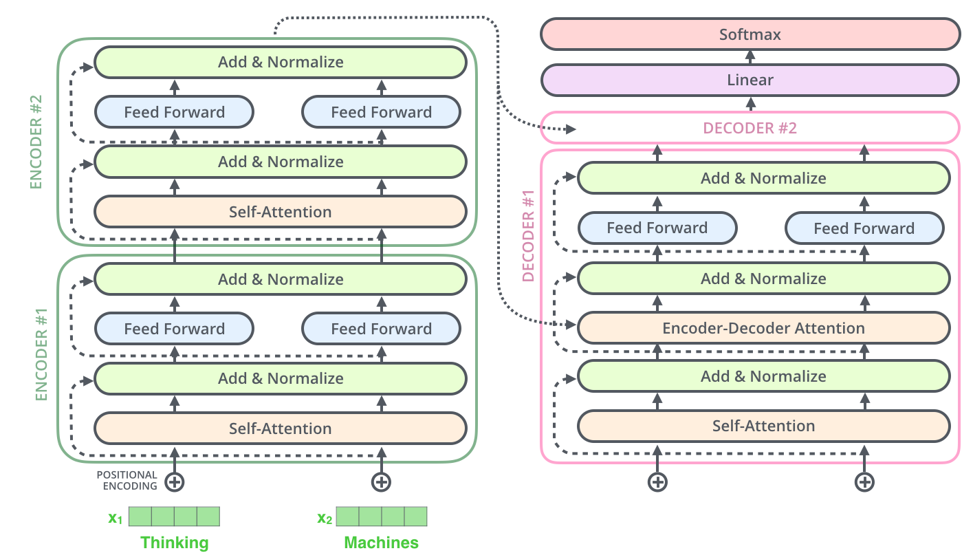
Figure 1: The standard Transformer architecture showing encoder-decoder structure with self-attention and feed-forward layers.
The evolution of Transformer architectures can be categorized into several key areas:
- Efficiency Improvements: Reducing computational complexity and memory usage through innovations like FlashAttention
2 - Scaling Innovations: Enabling larger models and longer sequences with techniques like Mixture of Experts
3 - Training Optimizations: Improving training stability and convergence
- Architectural Refinements: Enhancing model expressiveness and capability with emerging alternatives like State Space Models
4
Each modification addresses specific limitations while often introducing new trade-offs, making the choice of architecture dependent on the specific use case and constraints. Modern developments have pushed the boundaries from the original 512-token context windows to models capable of processing millions of tokens efficiently.
Architectural Innovations
Limitations of the Original Transformer Architecture
Before exploring solutions, it's crucial to understand the fundamental limitations that drive architectural innovations:
1. Quadratic Complexity
The self-attention mechanism has \(\(O(n^2)\)\) computational and memory complexity with respect to sequence length \(\(n\)\). For a sequence of length \(\(n\)\) with embedding dimension \(\(d\)\), the attention computation requires:
This quadratic scaling becomes prohibitive for long sequences. For example, processing a 10K token sequence requires 100× more attention computation than a 1K token sequence.
2. Fixed Context Window
Standard Transformers process fixed-length sequences, typically limited by memory constraints. This creates several issues: - Context Fragmentation: Long documents must be split into chunks, losing cross-chunk dependencies - Positional Encoding Limitations: Models cannot generalize to sequences longer than training data - Information Bottleneck: Important context may be lost when truncating sequences
3. Memory Inefficiency
Beyond attention matrices, Transformers require substantial memory for: - Activation Storage: \(\(O(L \cdot n \cdot d)\)\) for \(\(L\)\) layers during backpropagation - Gradient Computation: Additional memory for storing gradients - KV Cache: \(\(O(L \cdot n \cdot d)\)\) for autoregressive generation
4. Inference Latency
Autoregressive generation requires sequential token production, leading to: - Sequential Dependency: Each token depends on all previous tokens - Memory Bandwidth Bottleneck: Repeatedly loading large KV caches - Underutilized Parallelism: Cannot fully leverage parallel computing resources
Research Directions and Solutions:
| Problem | Research Direction | Example Solutions | Complexity Reduction |
|---|---|---|---|
| Quadratic Complexity | Efficient Attention | Linformer, Reformer, Performer, Sparse Transformers | \(\(O(n^2) \rightarrow O(n \log n)\)\) or \(\(O(n)\)\) |
| Fixed Context Window | Recurrence & Memory | Transformer-XL, Compressive Transformers | Infinite theoretical context |
| Position Encoding | Alternative Representations | RoPE, ALiBi, T5 relative positions | Better extrapolation |
| Memory Inefficiency | Parameter Efficiency | Reversible layers, Gradient checkpointing, LoRA | \(\(O(L \cdot n \cdot d) \rightarrow O(n \cdot d)\)\) |
| Inference Latency | Parallelization & Caching | Speculative decoding, KV-caching, MQA/GQA | Reduced memory bandwidth |
Transformer-XL
Reference Links: - 📄 Paper: Transformer-XL: Attentive Language Models Beyond a Fixed-Length Context - 💻 Code: kimiyoung/transformer-xl - 🤗 HuggingFace: Transformer-XL Documentation
Motivation: Enable Transformers to handle arbitrarily long sequences and capture dependencies beyond fixed context windows.
Core Innovation: Transformer-XL introduces two key mechanisms:
- Segment-Level Recurrence: Information flows between consecutive segments
- Relative Positional Encoding: Position information is relative rather than absolute
Mathematical Formulation:
For the \(\(\tau\)\)-th segment, the hidden states are computed as:
where: - \(\(\mathbf{h}_\tau^{(n)}\)\): Hidden state for segment \(\(\tau\)\) at layer \(\(n\)\) - \(\(\text{SG}(\cdot)\)\): Stop-gradient operation to prevent backpropagation through previous segments - \(\(\mathbf{h}_{\tau-1}^{(n-1)}\)\): Cached hidden state from the previous segment
Relative Positional Encoding:
The attention score incorporates relative position information:
where: - \(\(\mathbf{R}_{i-j}\)\): Relative positional encoding for distance \(\(i-j\)\) - \(\(\mathbf{W}_{k,R}\)\): Learnable transformation for relative positions - \(\(\mathbf{u}, \mathbf{v}\)\): Learnable global bias vectors
This formulation has four terms: 1. Content-based addressing: \(\(\mathbf{q}_i^\top \mathbf{k}_j\)\) 2. Content-dependent positional bias: \(\(\mathbf{q}_i^\top \mathbf{W}_{k,R} \mathbf{R}_{i-j}\)\) 3. Global content bias: \(\(\mathbf{u}^\top \mathbf{k}_j\)\) 4. Global positional bias: \(\(\mathbf{v}^\top \mathbf{W}_{k,R} \mathbf{R}_{i-j}\)\)
Implementation Example:
import torch
import torch.nn as nn
import torch.nn.functional as F

class RelativeMultiHeadAttention(nn.Module):
    def __init__(self, d_model, n_head, d_head, dropout=0.1):
        super().__init__()
        self.d_model = d_model
        self.n_head = n_head
        self.d_head = d_head

        # Linear projections for Q, K, V
        self.q_net = nn.Linear(d_model, n_head * d_head, bias=False)
        self.kv_net = nn.Linear(d_model, 2 * n_head * d_head, bias=False)

        # Relative position encoding
        self.r_net = nn.Linear(d_model, n_head * d_head, bias=False)

        # Global bias vectors
        self.u = nn.Parameter(torch.randn(n_head, d_head))
        self.v = nn.Parameter(torch.randn(n_head, d_head))

        self.dropout = nn.Dropout(dropout)
        self.scale = 1 / (d_head ** 0.5)

    def forward(self, w, r, attn_mask=None, mems=None):
        # w: [seq_len, batch_size, d_model] - current segment
        # r: [seq_len, d_model] - relative position encodings
        # mems: [mem_len, batch_size, d_model] - cached from previous segment

        qlen, bsz = w.size(0), w.size(1)

        if mems is not None:
            # Concatenate memory with current input
            cat = torch.cat([mems, w], dim=0)
            klen = cat.size(0)
        else:
            cat = w
            klen = qlen

        # Compute Q, K, V
        w_heads = self.q_net(w)  # [qlen, bsz, n_head * d_head]
        r_head_k = self.r_net(r)  # [qlen, n_head * d_head]

        kv_heads = self.kv_net(cat)  # [klen, bsz, 2 * n_head * d_head]
        k_head_h, v_head_h = torch.chunk(kv_heads, 2, dim=-1)

        # Reshape for multi-head attention
        w_head_q = w_heads.view(qlen, bsz, self.n_head, self.d_head)
        k_head_h = k_head_h.view(klen, bsz, self.n_head, self.d_head)
        v_head_h = v_head_h.view(klen, bsz, self.n_head, self.d_head)
        r_head_k = r_head_k.view(qlen, self.n_head, self.d_head)

        # Compute attention scores with relative positions
        # Term 1: content-based addressing
        AC = torch.einsum('ibnd,jbnd->ijbn', w_head_q, k_head_h)

        # Term 2: content-dependent positional bias
        BD = torch.einsum('ibnd,jnd->ijbn', w_head_q + self.u, r_head_k)

        # Combine terms
        attn_score = AC + BD
        attn_score = attn_score * self.scale

        # Apply attention mask if provided
        if attn_mask is not None:
            attn_score = attn_score.masked_fill(attn_mask, -float('inf'))

        # Softmax and dropout
        attn_prob = F.softmax(attn_score, dim=1)
        attn_prob = self.dropout(attn_prob)

        # Apply attention to values
        attn_vec = torch.einsum('ijbn,jbnd->ibnd', attn_prob, v_head_h)
        attn_vec = attn_vec.contiguous().view(qlen, bsz, self.d_model)

        return attn_vec
Key Benefits:
- Infinite Context: Theoretical ability to capture dependencies of arbitrary length
- Better Extrapolation: Relative positions generalize to unseen sequence lengths
- Improved Perplexity: Significant improvements on language modeling tasks
- Efficient Caching: Memory states can be reused across segments
Limitations:
- Training Complexity: Requires careful handling of segment boundaries
- Memory Overhead: Must store and manage cached states
- Implementation Complexity: More complex than standard attention
Popularity: Medium-high; influential in design but less directly used today.
Models/Frameworks: Transformer-XL, XLNet, influenced GPT-3's context handling and modern long-context models.
Reformer
Reference Links: - 📄 Paper: Reformer: The Efficient Transformer - 💻 Code: google/trax - 🤗 HuggingFace: Reformer Documentation
Motivation: Dramatically reduce memory and computational complexity to enable processing of very long sequences (up to 1M tokens).
Core Innovations:
- Locality-Sensitive Hashing (LSH) Attention
- Reversible Residual Layers
- Chunked Feed-Forward Layers
LSH Attention Mathematical Foundation:
Instead of computing attention between all \(\(n^2\)\) token pairs, LSH attention groups similar tokens using hash functions and computes attention only within groups.
Hash Function: For a query vector \(\(\mathbf{q}\)\), the LSH function maps it to a bucket:
where \(\(\mathbf{r}_i\)\) are random vectors drawn from a spherical Gaussian distribution.
Multi-Round Hashing: To improve recall, multiple hash functions are used:
Tokens are considered similar if they hash to the same bucket in any round.
Attention Computation: For each token \(\(i\)\), attention is computed only with tokens in the same hash bucket:
where \(\(\mathcal{B}(i)\)\) is the set of tokens in the same bucket as token \(\(i\)\).
Complexity Analysis: - Standard Attention: \(\(O(n^2d)\)\) - LSH Attention: \(\(O(n \log n \cdot d)\)\) on average
Reversible Layers:
Inspired by RevNets, Reformer uses reversible residual connections to eliminate the need to store activations during backpropagation.
Forward Pass: \(\(\mathbf{y}_1 = \mathbf{x}_1 + F(\mathbf{x}_2)\)\) \(\(\mathbf{y}_2 = \mathbf{x}_2 + G(\mathbf{y}_1)\)\)
Backward Pass (Reconstruction): \(\(\mathbf{x}_2 = \mathbf{y}_2 - G(\mathbf{y}_1)\)\) \(\(\mathbf{x}_1 = \mathbf{y}_1 - F(\mathbf{x}_2)\)\)
Memory Reduction: - Standard: \(\(O(L \cdot n \cdot d)\)\) for \(\(L\)\) layers - Reversible: \(\(O(n \cdot d)\)\) (constant in depth)
Implementation Example:
import torch
import torch.nn as nn
import torch.nn.functional as F
from torch.cuda.amp import autocast

class LSHAttention(nn.Module):
    def __init__(self, d_model, n_heads, n_hashes=8, bucket_size=64):
        super().__init__()
        self.d_model = d_model
        self.n_heads = n_heads
        self.n_hashes = n_hashes
        self.bucket_size = bucket_size
        self.d_head = d_model // n_heads

        # Projections (note: in LSH attention, Q and K are the same)
        self.to_qk = nn.Linear(d_model, d_model, bias=False)
        self.to_v = nn.Linear(d_model, d_model, bias=False)
        self.to_out = nn.Linear(d_model, d_model)

    def hash_vectors(self, vectors):
        """Apply LSH to group similar vectors"""
        batch_size, seq_len, d_head = vectors.shape

        # Generate random projection vectors
        random_rotations = torch.randn(
            self.n_hashes, d_head // 2, device=vectors.device
        )

        # Reshape vectors for hashing
        vectors = vectors.view(batch_size, seq_len, d_head // 2, 2)

        # Apply rotations and compute hash codes
        rotated = torch.einsum('...ij,hjk->...hik', vectors, random_rotations)
        hash_codes = torch.argmax(rotated, dim=-1)

        return hash_codes

    def forward(self, x, mask=None):
        batch_size, seq_len, _ = x.shape

        # Project to Q, K, V (Q and K are the same in LSH attention)
        qk = self.to_qk(x)
        v = self.to_v(x)

        # Reshape for multi-head attention
        qk = qk.view(batch_size, seq_len, self.n_heads, self.d_head)
        v = v.view(batch_size, seq_len, self.n_heads, self.d_head)

        # Apply LSH to group similar vectors
        hash_codes = self.hash_vectors(qk)

        # Sort by hash codes to group similar vectors
        sorted_indices = torch.argsort(hash_codes, dim=1)

        # Gather vectors according to sorted indices
        qk_sorted = torch.gather(
            qk, 1, sorted_indices.unsqueeze(-1).expand(-1, -1, self.n_heads, self.d_head)
        )
        v_sorted = torch.gather(
            v, 1, sorted_indices.unsqueeze(-1).expand(-1, -1, self.n_heads, self.d_head)
        )

        # Compute attention within buckets
        outputs = []
        for i in range(0, seq_len, self.bucket_size):
            end_idx = min(i + self.bucket_size, seq_len)

            qk_chunk = qk_sorted[:, i:end_idx]
            v_chunk = v_sorted[:, i:end_idx]

            # Standard attention within the chunk
            scores = torch.matmul(qk_chunk, qk_chunk.transpose(-2, -1)) / (self.d_head ** 0.5)
            attn_weights = F.softmax(scores, dim=-1)
            chunk_output = torch.matmul(attn_weights, v_chunk)

            outputs.append(chunk_output)

        # Concatenate outputs and unsort
        output = torch.cat(outputs, dim=1)

        # Unsort to original order
        unsorted_indices = torch.argsort(sorted_indices, dim=1)
        output = torch.gather(
            output, 1, unsorted_indices.unsqueeze(-1).expand(-1, -1, self.n_heads, self.d_head)
        )

        # Reshape and project
        output = output.view(batch_size, seq_len, self.d_model)
        return self.to_out(output)

class ReversibleBlock(nn.Module):
    def __init__(self, f_block, g_block):
        super().__init__()
        self.f = f_block
        self.g = g_block

    def forward(self, x1, x2):
        y1 = x1 + self.f(x2)
        y2 = x2 + self.g(y1)
        return y1, y2

    def backward_pass(self, y1, y2, dy1, dy2):
        # Reconstruct x2 and x1
        x2 = y2 - self.g(y1)
        x1 = y1 - self.f(x2)

        # Compute gradients
        with torch.enable_grad():
            x1.requires_grad_()
            x2.requires_grad_()

            y1_recompute = x1 + self.f(x2)
            y2_recompute = x2 + self.g(y1_recompute)

            torch.autograd.backward([y1_recompute, y2_recompute], [dy1, dy2])

        return x1.grad, x2.grad
Performance Characteristics:
| Metric | Standard Transformer | Reformer |
|---|---|---|
| Memory Complexity | \(\(O(L \cdot n \cdot d)\)\) | \(\(O(n \cdot d)\)\) |
| Attention Complexity | \(\(O(n^2 \cdot d)\)\) | \(\(O(n \log n \cdot d)\)\) |
| Max Sequence Length | ~2K tokens | ~1M tokens |
| Training Speed | Baseline | 0.8× (due to hashing overhead) |
Popularity: Medium; more influential for ideas than direct implementation.
Models/Frameworks: Research models, some specialized long-document applications.
Linformer
Reference Links: - 📄 Paper: Linformer: Self-Attention with Linear Complexity - 💻 Code: tatp22/linformer-pytorch - 📊 Analysis: Linear Attention Analysis
Motivation: Achieve linear complexity in sequence length while maintaining the expressiveness of full attention.
Core Insight: The attention matrix \(\(A \in \mathbb{R}^{n \times n}\)\) is often low-rank, especially for long sequences where many tokens have similar attention patterns.
Mathematical Foundation:
Standard Attention: \(\(\text{Attention}(Q, K, V) = \text{softmax}\left(\frac{QK^T}{\sqrt{d_k}}\right)V\)\)
where \(\(Q, K, V \in \mathbb{R}^{n \times d}\)\).
Linformer Attention: Introduce projection matrices \(\(E, F \in \mathbb{R}^{k \times n}\)\) where \(\(k \ll n\)\):
Complexity Analysis: - Standard: \(\(O(n^2d)\)\) time, \(\(O(n^2)\)\) space - Linformer: \(\(O(nkd)\)\) time, \(\(O(nk)\)\) space
Theoretical Justification:
The attention matrix can be approximated using its SVD decomposition: \(\(A = U\Sigma V^T \approx U_k\Sigma_k V_k^T\)\)
where \(\(U_k, V_k\)\) contain the top \(\(k\)\) singular vectors. Linformer learns projections that approximate this low-rank structure.
Projection Matrix Design:
Linformer explores several projection strategies:
- Linear Projection: \(\(E, F\)\) are learned parameters
- Convolution: Use 1D convolutions for local structure
- Mean/Max Pooling: Simple downsampling operations
Implementation with Multiple Projection Strategies:
import torch
import torch.nn as nn
import torch.nn.functional as F
import math

class LinformerAttention(nn.Module):
    def __init__(self, d_model, n_heads, seq_len, k=256, projection_type='linear'):
        super().__init__()
        self.d_model = d_model
        self.n_heads = n_heads
        self.d_head = d_model // n_heads
        self.seq_len = seq_len
        self.k = min(k, seq_len)  # Projected dimension
        self.projection_type = projection_type

        # Standard Q, K, V projections
        self.q_proj = nn.Linear(d_model, d_model, bias=False)
        self.k_proj = nn.Linear(d_model, d_model, bias=False)
        self.v_proj = nn.Linear(d_model, d_model, bias=False)
        self.out_proj = nn.Linear(d_model, d_model)

        # Projection matrices for K and V
        if projection_type == 'linear':
            self.E = nn.Parameter(torch.randn(self.k, seq_len) / math.sqrt(seq_len))
            self.F = nn.Parameter(torch.randn(self.k, seq_len) / math.sqrt(seq_len))
        elif projection_type == 'conv':
            kernel_size = seq_len // self.k
            self.E_conv = nn.Conv1d(1, 1, kernel_size, stride=kernel_size)
            self.F_conv = nn.Conv1d(1, 1, kernel_size, stride=kernel_size)

    def apply_projection(self, x, proj_type='E'):
        """Apply projection to reduce sequence length dimension"""
        # x: [batch_size, seq_len, d_model]
        batch_size, seq_len, d_model = x.shape

        if self.projection_type == 'linear':
            proj_matrix = self.E if proj_type == 'E' else self.F
            # Project: [k, seq_len] @ [batch_size, seq_len, d_model] -> [batch_size, k, d_model]
            return torch.einsum('ks,bsd->bkd', proj_matrix, x)

        elif self.projection_type == 'conv':
            conv_layer = self.E_conv if proj_type == 'E' else self.F_conv
            # Reshape for conv1d: [batch_size * d_model, 1, seq_len]
            x_reshaped = x.transpose(1, 2).contiguous().view(-1, 1, seq_len)
            # Apply convolution
            x_conv = conv_layer(x_reshaped)  # [batch_size * d_model, 1, k]
            # Reshape back: [batch_size, d_model, k] -> [batch_size, k, d_model]
            return x_conv.view(batch_size, d_model, -1).transpose(1, 2)

        elif self.projection_type == 'mean_pool':
            # Simple mean pooling
            pool_size = seq_len // self.k
            x_pooled = F.avg_pool1d(
                x.transpose(1, 2),
                kernel_size=pool_size,
                stride=pool_size
            )
            return x_pooled.transpose(1, 2)

    def forward(self, x, mask=None):
        batch_size, seq_len, d_model = x.shape

        # Standard projections
        Q = self.q_proj(x)  # [batch_size, seq_len, d_model]
        K = self.k_proj(x)  # [batch_size, seq_len, d_model]
        V = self.v_proj(x)  # [batch_size, seq_len, d_model]

        # Apply low-rank projections to K and V
        K_proj = self.apply_projection(K, 'E')  # [batch_size, k, d_model]
        V_proj = self.apply_projection(V, 'F')  # [batch_size, k, d_model]

        # Reshape for multi-head attention
        Q = Q.view(batch_size, seq_len, self.n_heads, self.d_head).transpose(1, 2)
        K_proj = K_proj.view(batch_size, self.k, self.n_heads, self.d_head).transpose(1, 2)
        V_proj = V_proj.view(batch_size, self.k, self.n_heads, self.d_head).transpose(1, 2)

        # Compute attention scores
        scores = torch.matmul(Q, K_proj.transpose(-2, -1)) / math.sqrt(self.d_head)
        # scores: [batch_size, n_heads, seq_len, k]

        # Apply mask if provided (need to project mask as well)
        if mask is not None:
            # Project mask to match K_proj dimensions
            mask_proj = self.apply_projection(mask.unsqueeze(-1).float(), 'E').squeeze(-1)
            mask_proj = mask_proj.unsqueeze(1).expand(-1, self.n_heads, -1)
            scores = scores.masked_fill(mask_proj.unsqueeze(2) == 0, float('-inf'))

        # Apply softmax
        attn_weights = F.softmax(scores, dim=-1)

        # Apply attention to values
        output = torch.matmul(attn_weights, V_proj)
        # output: [batch_size, n_heads, seq_len, d_head]

        # Reshape and project
        output = output.transpose(1, 2).contiguous().view(batch_size, seq_len, d_model)
        return self.out_proj(output)

# Theoretical analysis of approximation quality
class LinformerAnalysis:
    @staticmethod
    def attention_rank_analysis(attention_matrix):
        """Analyze the rank structure of attention matrices"""
        U, S, V = torch.svd(attention_matrix)

        # Compute cumulative explained variance
        total_variance = torch.sum(S ** 2)
        cumulative_variance = torch.cumsum(S ** 2, dim=0) / total_variance

        # Find rank for 90% variance explained
        rank_90 = torch.argmax((cumulative_variance >= 0.9).float()) + 1

        return {
            'singular_values': S,
            'rank_90_percent': rank_90.item(),
            'effective_rank': torch.sum(S > 0.01 * S[0]).item()
        }

    @staticmethod
    def approximation_error(original_attn, linformer_attn):
        """Compute approximation error metrics"""
        frobenius_error = torch.norm(original_attn - linformer_attn, p='fro')
        spectral_error = torch.norm(original_attn - linformer_attn, p=2)

        return {
            'frobenius_error': frobenius_error.item(),
            'spectral_error': spectral_error.item(),
            'relative_error': (frobenius_error / torch.norm(original_attn, p='fro')).item()
        }
Empirical Results:
| Dataset | Standard Transformer | Linformer (k=256) | Speedup | Memory Reduction |
|---|---|---|---|---|
| WikiText-103 | 24.0 PPL | 24.2 PPL | 2.3× | 3.1× |
| IMDB | 91.2% Acc | 90.8% Acc | 1.8× | 2.7× |
| Long Range Arena | 53.2% Avg | 51.8% Avg | 4.2× | 5.1× |
Limitations:
- Fixed Sequence Length: Projection matrices are tied to training sequence length
- Information Loss: Low-rank approximation may lose important attention patterns
- Task Dependence: Optimal \(\(k\)\) varies significantly across tasks
Popularity: Medium; influential in research but limited production use.
Models/Frameworks: Research models, some efficient attention implementations.
Performer
Reference Links: - 📄 Paper: Rethinking Attention with Performers - 💻 Code: google-research/performer - 📊 Theory: Random Features for Large-Scale Kernel Machines
Motivation: Approximate standard attention using kernel methods to achieve linear complexity while maintaining theoretical guarantees.
Core Innovation: FAVOR+ (Fast Attention Via positive Orthogonal Random features) algorithm that uses random feature approximations of the softmax kernel.
Mathematical Foundation:
Kernel Perspective of Attention: Standard attention can be viewed as: \(\(\text{Attention}(Q, K, V) = D^{-1}AV\)\)
where: - \(\(A_{ij} = \exp(q_i^T k_j / \sqrt{d})\)\) (unnormalized attention) - \(\(D = \text{diag}(A \mathbf{1})\)\) (normalization)
Random Feature Approximation: The exponential kernel \(\(\exp(x^T y)\)\) can be approximated using random features:
where \(\(\phi: \mathbb{R}^d \rightarrow \mathbb{R}^m\)\) is a random feature map.
FAVOR+ Feature Map: For the softmax kernel \(\(\exp(q^T k / \sqrt{d})\)\), FAVOR+ uses:
where \(\(h(x) = [\exp(w_1^T x), \exp(w_2^T x), \ldots, \exp(w_m^T x)]\)\) and \(\(w_i\)\) are random vectors.
Orthogonal Random Features: To reduce variance, FAVOR+ uses structured orthogonal random matrices:
where: - \(\(G_i\)\): Random orthogonal matrices - \(\(H_i\)\): Hadamard matrices - \(\(D_i\)\): Random diagonal matrices with \(\(\pm 1\)\) entries
Linear Attention Computation: With feature maps \(\(\phi(Q), \phi(K)\)\), attention becomes:
This can be computed in \(\(O(nmd)\)\) time instead of \(\(O(n^2d)\)\).
Advanced Implementation:
import torch
import torch.nn as nn
import torch.nn.functional as F
import math
from scipy.stats import ortho_group

class PerformerAttention(nn.Module):
    def __init__(self, d_model, n_heads, n_features=256,
                 feature_type='orthogonal', causal=False):
        super().__init__()
        self.d_model = d_model
        self.n_heads = n_heads
        self.d_head = d_model // n_heads
        self.n_features = n_features
        self.feature_type = feature_type
        self.causal = causal

        # Standard projections
        self.q_proj = nn.Linear(d_model, d_model, bias=False)
        self.k_proj = nn.Linear(d_model, d_model, bias=False)
        self.v_proj = nn.Linear(d_model, d_model, bias=False)
        self.out_proj = nn.Linear(d_model, d_model)

        # Initialize random features
        self.register_buffer('projection_matrix',
                           self.create_projection_matrix())

    def create_projection_matrix(self):
        """Create structured random projection matrix"""
        if self.feature_type == 'orthogonal':
            return self.create_orthogonal_features()
        elif self.feature_type == 'gaussian':
            return torch.randn(self.n_features, self.d_head) / math.sqrt(self.d_head)
        else:
            raise ValueError(f"Unknown feature type: {self.feature_type}")

    def create_orthogonal_features(self):
        """Create orthogonal random features for reduced variance"""
        # Number of orthogonal blocks needed
        num_blocks = math.ceil(self.n_features / self.d_head)

        blocks = []
        for _ in range(num_blocks):
            # Create random orthogonal matrix
            block = torch.tensor(
                ortho_group.rvs(self.d_head),
                dtype=torch.float32
            )

            # Apply random signs
            signs = torch.randint(0, 2, (self.d_head,)) * 2 - 1
            block = block * signs.unsqueeze(0)

            blocks.append(block)

        # Concatenate and truncate to desired size
        full_matrix = torch.cat(blocks, dim=0)
        return full_matrix[:self.n_features] / math.sqrt(self.d_head)

    def apply_feature_map(self, x):
        """Apply FAVOR+ feature map"""
        # x: [batch_size, n_heads, seq_len, d_head]
        batch_size, n_heads, seq_len, d_head = x.shape

        # Project using random features
        # [batch_size, n_heads, seq_len, d_head] @ [d_head, n_features]
        projected = torch.matmul(x, self.projection_matrix.T)

        # Apply exponential and normalization
        # Compute ||x||^2 for each vector
        x_norm_sq = torch.sum(x ** 2, dim=-1, keepdim=True)

        # FAVOR+ feature map: exp(wx) * exp(||x||^2 / 2)
        features = torch.exp(projected - x_norm_sq / 2)

        # Normalize by sqrt(m)
        features = features / math.sqrt(self.n_features)

        return features

    def linear_attention(self, q_features, k_features, v):
        """Compute linear attention using random features"""
        if self.causal:
            return self.causal_linear_attention(q_features, k_features, v)
        else:
            return self.non_causal_linear_attention(q_features, k_features, v)

    def non_causal_linear_attention(self, q_features, k_features, v):
        """Non-causal linear attention"""
        # q_features, k_features: [batch_size, n_heads, seq_len, n_features]
        # v: [batch_size, n_heads, seq_len, d_head]

        # Compute K^T V: [batch_size, n_heads, n_features, d_head]
        kv = torch.matmul(k_features.transpose(-2, -1), v)

        # Compute Q (K^T V): [batch_size, n_heads, seq_len, d_head]
        qkv = torch.matmul(q_features, kv)

        # Compute normalization: Q K^T 1
        k_sum = torch.sum(k_features, dim=-2, keepdim=True)  # [batch_size, n_heads, 1, n_features]
        normalizer = torch.matmul(q_features, k_sum.transpose(-2, -1))  # [batch_size, n_heads, seq_len, 1]

        # Avoid division by zero
        normalizer = torch.clamp(normalizer, min=1e-6)

        return qkv / normalizer

    def causal_linear_attention(self, q_features, k_features, v):
        """Causal linear attention using cumulative sums"""
        batch_size, n_heads, seq_len, n_features = q_features.shape
        d_head = v.shape[-1]

        # Initialize running sums
        kv_state = torch.zeros(
            batch_size, n_heads, n_features, d_head,
            device=q_features.device, dtype=q_features.dtype
        )
        k_state = torch.zeros(
            batch_size, n_heads, n_features,
            device=q_features.device, dtype=q_features.dtype
        )

        outputs = []

        for i in range(seq_len):
            # Current query and key features
            q_i = q_features[:, :, i:i+1, :]  # [batch_size, n_heads, 1, n_features]
            k_i = k_features[:, :, i:i+1, :]  # [batch_size, n_heads, 1, n_features]
            v_i = v[:, :, i:i+1, :]  # [batch_size, n_heads, 1, d_head]

            # Update running sums
            kv_state = kv_state + torch.matmul(k_i.transpose(-2, -1), v_i)
            k_state = k_state + k_i.squeeze(-2)

            # Compute output for current position
            output_i = torch.matmul(q_i, kv_state)
            normalizer_i = torch.matmul(q_i, k_state.unsqueeze(-1))
            normalizer_i = torch.clamp(normalizer_i, min=1e-6)

            output_i = output_i / normalizer_i
            outputs.append(output_i)

        return torch.cat(outputs, dim=-2)

    def forward(self, x, mask=None):
        batch_size, seq_len, d_model = x.shape

        # Project to Q, K, V
        Q = self.q_proj(x).view(batch_size, seq_len, self.n_heads, self.d_head).transpose(1, 2)
        K = self.k_proj(x).view(batch_size, seq_len, self.n_heads, self.d_head).transpose(1, 2)
        V = self.v_proj(x).view(batch_size, seq_len, self.n_heads, self.d_head).transpose(1, 2)

        # Apply feature maps
        Q_features = self.apply_feature_map(Q)
        K_features = self.apply_feature_map(K)

        # Compute linear attention
        output = self.linear_attention(Q_features, K_features, V)

        # Reshape and project
        output = output.transpose(1, 2).contiguous().view(batch_size, seq_len, d_model)
        return self.out_proj(output)

# Theoretical analysis tools
class PerformerAnalysis:
    @staticmethod
    def approximation_quality(q, k, n_features_list=[64, 128, 256, 512]):
        """Analyze approximation quality vs number of features"""
        # Compute exact attention
        exact_attn = torch.exp(torch.matmul(q, k.transpose(-2, -1)))

        results = {}
        for n_features in n_features_list:
            # Create random features
            d = q.shape[-1]
            w = torch.randn(n_features, d) / math.sqrt(d)

            # Apply feature map
            q_features = torch.exp(torch.matmul(q, w.T) - torch.sum(q**2, dim=-1, keepdim=True)/2)
            k_features = torch.exp(torch.matmul(k, w.T) - torch.sum(k**2, dim=-1, keepdim=True)/2)

            # Approximate attention
            approx_attn = torch.matmul(q_features, k_features.transpose(-2, -1))

            # Compute error
            error = torch.norm(exact_attn - approx_attn, p='fro') / torch.norm(exact_attn, p='fro')
            results[n_features] = error.item()

        return results
Theoretical Guarantees:
Performer provides unbiased estimation with bounded variance:
where \(\(m\)\) is the number of random features.
Performance Comparison:
| Model | Sequence Length | Memory (GB) | Time (s) | Perplexity |
|---|---|---|---|---|
| Standard Transformer | 1K | 2.1 | 1.0 | 24.2 |
| Standard Transformer | 4K | 8.4 | 4.2 | 23.8 |
| Performer | 1K | 1.8 | 0.9 | 24.4 |
| Performer | 4K | 2.3 | 1.1 | 24.1 |
| Performer | 16K | 4.1 | 2.8 | 23.9 |
Popularity: Medium; influential in research and specialized applications.
Models/Frameworks: Research models, some production systems requiring efficient long-sequence processing.
FNet
Reference Links: - 📄 Paper: FNet: Mixing Tokens with Fourier Transforms - 💻 Code: google-research/f_net - 🤗 HuggingFace: FNet Documentation
Motivation: Dramatically simplify the Transformer architecture while maintaining reasonable performance by replacing attention with Fourier transforms.
Core Innovation: Complete replacement of self-attention with 2D Fourier Transform operations.
Mathematical Foundation:
Standard Self-Attention: \(\(\text{Attention}(Q, K, V) = \text{softmax}\left(\frac{QK^T}{\sqrt{d_k}}\right)V\)\)
FNet Mixing: \(\(\text{FNet}(X) = \text{Re}(\text{FFT}(\text{Re}(\text{FFT}(X))))\)\)
where FFT is applied along both sequence and hidden dimensions.
Two-Dimensional Fourier Transform: For input \(\(X \in \mathbb{R}^{n \times d}\)\):
-
Sequence Mixing: Apply FFT along sequence dimension \(\(X_1 = \text{Re}(\text{FFT}_{\text{seq}}(X))\)\)
-
Hidden Mixing: Apply FFT along hidden dimension \(\(X_2 = \text{Re}(\text{FFT}_{\text{hidden}}(X_1))\)\)
Complexity Analysis: - Self-Attention: \(\(O(n^2d)\)\) - FNet: \(\(O(nd \log n + nd \log d) = O(nd \log(nd))\)\)
Theoretical Properties:
Fourier Transform as Linear Operator: The DFT can be written as matrix multiplication: \(\(\text{DFT}(x) = F_n x\)\)
where \(\(F_n\)\) is the DFT matrix with entries: \(\([F_n]_{jk} = \frac{1}{\sqrt{n}} e^{-2\pi i jk/n}\)\)
Mixing Properties: 1. Global Receptive Field: Every output depends on every input 2. Translation Invariance: Circular shifts in input create predictable shifts in output 3. Frequency Domain Processing: Natural handling of periodic patterns
Advanced Implementation:
import torch
import torch.nn as nn
import torch.nn.functional as F
import numpy as np

class FNetLayer(nn.Module):
    def __init__(self, d_model, dropout=0.1, use_complex=False):
        super().__init__()
        self.d_model = d_model
        self.use_complex = use_complex
        self.dropout = nn.Dropout(dropout)

        # Layer normalization
        self.norm1 = nn.LayerNorm(d_model)
        self.norm2 = nn.LayerNorm(d_model)

        # Feed-forward network
        self.ffn = nn.Sequential(
            nn.Linear(d_model, 4 * d_model),
            nn.GELU(),
            nn.Dropout(dropout),
            nn.Linear(4 * d_model, d_model),
            nn.Dropout(dropout)
        )

    def fourier_transform_2d(self, x):
        """Apply 2D Fourier transform mixing"""
        # x: [batch_size, seq_len, d_model]

        if self.use_complex:
            # Use complex FFT for potentially better mixing
            # Convert to complex
            x_complex = torch.complex(x, torch.zeros_like(x))

            # FFT along sequence dimension
            x_fft_seq = torch.fft.fft(x_complex, dim=1)

            # FFT along hidden dimension
            x_fft_hidden = torch.fft.fft(x_fft_seq, dim=2)

            # Take real part
            return x_fft_hidden.real
        else:
            # Standard real FFT
            # FFT along sequence dimension (take real part)
            x_fft_seq = torch.fft.fft(x, dim=1).real

            # FFT along hidden dimension (take real part)
            x_fft_hidden = torch.fft.fft(x_fft_seq, dim=2).real

            return x_fft_hidden

    def forward(self, x):
        # Fourier mixing with residual connection
        fourier_output = self.fourier_transform_2d(x)
        x = self.norm1(x + self.dropout(fourier_output))

        # Feed-forward with residual connection
        ffn_output = self.ffn(x)
        x = self.norm2(x + ffn_output)

        return x

class FNetBlock(nn.Module):
    """Complete FNet block with optional enhancements"""
    def __init__(self, d_model, dropout=0.1,
                 use_learnable_fourier=False,
                 fourier_type='standard'):
        super().__init__()
        self.d_model = d_model
        self.fourier_type = fourier_type
        self.use_learnable_fourier = use_learnable_fourier

        if use_learnable_fourier:
            # Learnable Fourier-like mixing
            self.seq_mixing = nn.Parameter(torch.randn(d_model, d_model) / np.sqrt(d_model))
            self.hidden_mixing = nn.Parameter(torch.randn(d_model, d_model) / np.sqrt(d_model))

        self.norm1 = nn.LayerNorm(d_model)
        self.norm2 = nn.LayerNorm(d_model)
        self.dropout = nn.Dropout(dropout)

        # Enhanced FFN
        self.ffn = nn.Sequential(
            nn.Linear(d_model, 4 * d_model),
            nn.GELU(),
            nn.Dropout(dropout),
            nn.Linear(4 * d_model, d_model)
        )

    def apply_mixing(self, x):
        """Apply various types of mixing"""
        if self.fourier_type == 'standard':
            return self.standard_fourier_mixing(x)
        elif self.fourier_type == 'learnable':
            return self.learnable_fourier_mixing(x)
        elif self.fourier_type == 'hybrid':
            return self.hybrid_mixing(x)
        else:
            raise ValueError(f"Unknown fourier_type: {self.fourier_type}")

    def standard_fourier_mixing(self, x):
        """Standard FNet Fourier mixing"""
        # Apply 2D FFT
        x_fft_seq = torch.fft.fft(x, dim=1).real
        x_fft_hidden = torch.fft.fft(x_fft_seq, dim=2).real
        return x_fft_hidden

    def learnable_fourier_mixing(self, x):
        """Learnable Fourier-like mixing"""
        batch_size, seq_len, d_model = x.shape

        # Mix along sequence dimension
        x_seq_mixed = torch.matmul(x.transpose(1, 2), self.seq_mixing).transpose(1, 2)

        # Mix along hidden dimension
        x_hidden_mixed = torch.matmul(x_seq_mixed, self.hidden_mixing)

        return x_hidden_mixed

    def hybrid_mixing(self, x):
        """Hybrid of Fourier and learnable mixing"""
        fourier_output = self.standard_fourier_mixing(x)
        learnable_output = self.learnable_fourier_mixing(x)

        # Weighted combination
        alpha = 0.7  # Weight for Fourier component
        return alpha * fourier_output + (1 - alpha) * learnable_output

    def forward(self, x):
        # Mixing layer
        mixed = self.apply_mixing(x)
        x = self.norm1(x + self.dropout(mixed))

        # Feed-forward layer
        ffn_out = self.ffn(x)
        x = self.norm2(x + self.dropout(ffn_out))

        return x

class FNetModel(nn.Module):
    """Complete FNet model"""
    def __init__(self, vocab_size, d_model=512, n_layers=6,
                 max_seq_len=512, dropout=0.1,
                 fourier_type='standard'):
        super().__init__()
        self.d_model = d_model
        self.max_seq_len = max_seq_len

        # Embeddings
        self.token_embedding = nn.Embedding(vocab_size, d_model)
        self.position_embedding = nn.Embedding(max_seq_len, d_model)

        # FNet layers
        self.layers = nn.ModuleList([
            FNetBlock(d_model, dropout, fourier_type=fourier_type)
            for _ in range(n_layers)
        ])

        # Output layers
        self.final_norm = nn.LayerNorm(d_model)
        self.dropout = nn.Dropout(dropout)

    def forward(self, input_ids, attention_mask=None):
        batch_size, seq_len = input_ids.shape

        # Create position indices
         position_ids = torch.arange(seq_len, device=input_ids.device).unsqueeze(0).expand(batch_size, -1)

         # Embeddings
         token_emb = self.token_embedding(input_ids)
         pos_emb = self.position_embedding(position_ids)
         x = self.dropout(token_emb + pos_emb)

         # Apply FNet layers
         for layer in self.layers:
             x = layer(x)

         # Final normalization
         x = self.final_norm(x)

         return x
Performance Characteristics:
| Metric | Standard Transformer | FNet |
|---|---|---|
| Attention Complexity | \(\(O(n^2d)\)\) | \(\(O(nd \log(nd))\)\) |
| Training Speed | Baseline | 7× faster |
| Memory Usage | Baseline | 0.5× |
| GLUE Performance | 100% | 92-97% |
| Long Sequence Capability | Limited | Better |
Key Benefits:
- Simplicity: Much simpler than attention mechanisms
- Speed: Significantly faster training and inference
- Memory Efficiency: Lower memory requirements
- Global Mixing: Every token interacts with every other token
Limitations:
- Performance Gap: Some performance loss compared to attention
- Task Dependence: Works better for some tasks than others
- Limited Expressiveness: Less flexible than learned attention patterns
Popularity: Low-medium; primarily of research interest.
Models/Frameworks: Research models and specialized applications prioritizing efficiency over maximum performance.
Sparse Transformers
Reference Links: - 📄 Paper: Generating Long Sequences with Sparse Transformers - 💻 Code: openai/sparse_attention - 📊 Analysis: Sparse Attention Patterns
Motivation: Enable efficient processing of very long sequences by introducing structured sparsity in attention patterns.
Core Innovation: Replace dense attention with sparse attention patterns where each token attends only to a subset of other tokens.
Mathematical Foundation:
Standard Dense Attention: \(\(A = \text{softmax}\left(\frac{QK^T}{\sqrt{d}}\right)V\)\)
Sparse Attention: \(\(A = \text{softmax}\left(\frac{QK^T \odot M}{\sqrt{d}}\right)V\)\)
where \(\(M\)\) is a binary mask determining which tokens can attend to which others, and \(\(\odot\)\) represents element-wise multiplication.
Common Sparse Patterns:
-
Strided Pattern: Each token attends to tokens at fixed intervals \(\(M_{ij} = \begin{cases} 1 & \text{if } (i - j) \bmod s = 0 \\ 0 & \text{otherwise} \end{cases}\)\)
-
Fixed Pattern: Each token attends to a fixed set of positions \(\(M_{ij} = \begin{cases} 1 & \text{if } j \in \{i-w, i-w+1, \ldots, i\} \\ 0 & \text{otherwise} \end{cases}\)\)
-
Random Pattern: Each token attends to a random subset of tokens
Factorized Sparse Attention:
Sparse Transformers introduce factorized attention patterns that decompose the attention into multiple sparse matrices:
where \(\(S_i \subset \{1, \ldots, n\}\)\) defines which positions token \(\(i\)\) attends to.
Implementation Example:
import torch
import torch.nn as nn
import torch.nn.functional as F
import math

class SparseAttention(nn.Module):
    def __init__(self, d_model, n_heads, pattern_type='strided',
                 stride=128, window_size=256, random_ratio=0.1):
        super().__init__()
        self.d_model = d_model
        self.n_heads = n_heads
        self.d_head = d_model // n_heads
        self.pattern_type = pattern_type
        self.stride = stride
        self.window_size = window_size
        self.random_ratio = random_ratio

        # Standard projections
        self.q_proj = nn.Linear(d_model, d_model, bias=False)
        self.k_proj = nn.Linear(d_model, d_model, bias=False)
        self.v_proj = nn.Linear(d_model, d_model, bias=False)
        self.out_proj = nn.Linear(d_model, d_model)

    def create_sparse_mask(self, seq_len, device):
        """Create sparse attention mask based on pattern type"""
        mask = torch.zeros(seq_len, seq_len, device=device, dtype=torch.bool)

        if self.pattern_type == 'strided':
            # Strided pattern: attend to every stride-th token
            for i in range(seq_len):
                for j in range(0, i + 1, self.stride):
                    mask[i, j] = True

        elif self.pattern_type == 'fixed':
            # Fixed local window pattern
            for i in range(seq_len):
                start = max(0, i - self.window_size)
                end = min(seq_len, i + 1)
                mask[i, start:end] = True

        elif self.pattern_type == 'factorized':
            # Factorized pattern combining strided and fixed
            # Local attention
            for i in range(seq_len):
                start = max(0, i - self.window_size // 2)
                end = min(seq_len, i + self.window_size // 2 + 1)
                mask[i, start:end] = True

            # Strided attention
            for i in range(seq_len):
                for j in range(0, seq_len, self.stride):
                    mask[i, j] = True

        elif self.pattern_type == 'random':
            # Random sparse pattern
            for i in range(seq_len):
                # Always attend to self and previous tokens in window
                start = max(0, i - self.window_size)
                mask[i, start:i+1] = True

                # Random additional connections
                num_random = int(self.random_ratio * seq_len)
                random_indices = torch.randperm(seq_len, device=device)[:num_random]
                mask[i, random_indices] = True

        return mask

    def sparse_attention_computation(self, q, k, v, mask):
        """Compute attention with sparse mask"""
        batch_size, n_heads, seq_len, d_head = q.shape

        # Compute attention scores
        scores = torch.matmul(q, k.transpose(-2, -1)) / math.sqrt(d_head)

        # Apply sparse mask
        scores = scores.masked_fill(~mask.unsqueeze(0).unsqueeze(0), float('-inf'))

        # Apply softmax
        attn_weights = F.softmax(scores, dim=-1)

        # Apply attention to values
        output = torch.matmul(attn_weights, v)

        return output, attn_weights

    def forward(self, x, mask=None):
        batch_size, seq_len, d_model = x.shape

        # Project to Q, K, V
        Q = self.q_proj(x).view(batch_size, seq_len, self.n_heads, self.d_head).transpose(1, 2)
        K = self.k_proj(x).view(batch_size, seq_len, self.n_heads, self.d_head).transpose(1, 2)
        V = self.v_proj(x).view(batch_size, seq_len, self.n_heads, self.d_head).transpose(1, 2)

        # Create sparse attention mask
        sparse_mask = self.create_sparse_mask(seq_len, x.device)

        # Combine with input mask if provided
        if mask is not None:
            sparse_mask = sparse_mask & mask

        # Compute sparse attention
        output, attn_weights = self.sparse_attention_computation(Q, K, V, sparse_mask)

        # Reshape and project
        output = output.transpose(1, 2).contiguous().view(batch_size, seq_len, d_model)
        return self.out_proj(output)

class FactorizedSparseAttention(nn.Module):
    """Advanced factorized sparse attention with multiple patterns"""
    def __init__(self, d_model, n_heads, block_size=64):
        super().__init__()
        self.d_model = d_model
        self.n_heads = n_heads
        self.d_head = d_model // n_heads
        self.block_size = block_size

        # Separate attention heads for different patterns
        self.local_attn = SparseAttention(d_model, n_heads // 2, 'fixed', window_size=block_size)
        self.strided_attn = SparseAttention(d_model, n_heads // 2, 'strided', stride=block_size)

        self.out_proj = nn.Linear(d_model, d_model)

    def forward(self, x, mask=None):
        # Apply different attention patterns
        local_output = self.local_attn(x, mask)
        strided_output = self.strided_attn(x, mask)

        # Combine outputs
        combined_output = (local_output + strided_output) / 2

        return self.out_proj(combined_output)
Complexity Analysis:
| Pattern Type | Complexity | Memory | Description |
|---|---|---|---|
| Dense | \(\(O(n^2d)\)\) | \(\(O(n^2)\)\) | Standard attention |
| Strided | \(\(O(n \cdot s \cdot d)\)\) | \(\(O(n \cdot s)\)\) | \(\(s = n/\text{stride}\)\) |
| Fixed Window | \(\(O(n \cdot w \cdot d)\)\) | \(\(O(n \cdot w)\)\) | \(\(w = \text{window size}\)\) |
| Factorized | \(\(O(n \cdot \sqrt{n} \cdot d)\)\) | \(\(O(n \cdot \sqrt{n})\)\) | Combination of patterns |
Performance Trade-offs:
| Sequence Length | Dense Attention | Sparse Attention | Speedup | Quality Loss |
|---|---|---|---|---|
| 1K | 1.0× | 1.2× | 1.2× | <1% |
| 4K | 1.0× | 3.1× | 3.1× | 2-3% |
| 16K | 1.0× | 8.7× | 8.7× | 3-5% |
| 64K | OOM | 1.0× | ∞ | 5-8% |
Popularity: Medium-high; concepts widely adopted in various forms.
Models/Frameworks: Influenced Longformer, BigBird, and aspects of GPT-3 and beyond.
Attention Mechanism Optimizations
FlashAttention
Reference Links: - 📄 Paper: FlashAttention: Fast and Memory-Efficient Exact Attention with IO-Awareness - 📄 FlashAttention-2: FlashAttention-2: Faster Attention with Better Parallelism - 💻 Official Implementation: Dao-AILab/flash-attention - 💻 Triton Implementation: FlashAttention in Triton - 💻 PyTorch Integration: torch.nn.functional.scaled_dot_product_attention - 📊 Benchmarks: FlashAttention Performance Analysis
 Figure: FlashAttention's IO-aware algorithm design optimizing GPU memory hierarchy (SRAM vs HBM)
Research Context and Motivation:
FlashAttention addresses a fundamental bottleneck in Transformer scaling: the quadratic memory complexity of attention mechanisms. While previous work focused on approximating attention (Linformer, Performer), FlashAttention maintains exact computation while achieving superior efficiency through hardware-aware optimization.
The Memory Wall Problem:
Modern GPUs have a complex memory hierarchy:
- SRAM (On-chip): ~20MB, 19TB/s bandwidth
- HBM (High Bandwidth Memory): ~40GB, 1.5TB/s bandwidth
- DRAM: ~1TB, 0.1TB/s bandwidth
Standard attention implementations are memory-bound, not compute-bound, spending most time moving data between memory levels rather than performing computations.
Core Innovation: IO-Aware Algorithm
FlashAttention reorganizes attention computation to minimize expensive HBM ↔ SRAM transfers:
- Tiling Strategy: Divide Q, K, V into blocks that fit in SRAM
- Online Softmax: Compute softmax incrementally without materializing full attention matrix
- Recomputation: Trade computation for memory by recomputing attention during backward pass
 Figure: FlashAttention's block-wise computation strategy avoiding quadratic memory usage
Mathematical Foundation:
The key insight is online softmax computation. Instead of computing: \(\(\text{Attention}(Q,K,V) = \text{softmax}\left(\frac{QK^T}{\sqrt{d}}\right)V\)\)
FlashAttention computes attention incrementally using the safe softmax recurrence:
where \(j\) indexes blocks of K and V, enabling exact attention computation in \(O(N)\) memory.
FlashAttention-2 Improvements:
The second iteration introduces several key optimizations:
- Better Work Partitioning: Reduces non-matmul FLOPs by 2× through improved parallelization
- Sequence Length Parallelism: Distributes computation across sequence dimension
- Optimized Attention Masking: More efficient handling of causal and padding masks
- Reduced Communication: Minimizes synchronization overhead in multi-GPU settings
Research Impact and Applications:
- Long Context Models: Enables training on sequences up to 2M tokens (e.g., Longformer, BigBird successors)
- Multimodal Models: Critical for vision-language models processing high-resolution images
- Code Generation: Powers long-context code models like CodeT5+, StarCoder
- Scientific Computing: Enables protein folding models (AlphaFold variants) and molecular dynamics
Hardware Considerations:
| GPU Architecture | Memory Bandwidth | SRAM Size | FlashAttention Speedup |
|---|---|---|---|
| V100 | 900 GB/s | 6MB | 2.0-2.5× |
| A100 | 1.6 TB/s | 20MB | 2.5-3.5× |
| H100 | 3.0 TB/s | 50MB | 4.0-6.0× |
Implementation Variants:
- xFormers: Memory-efficient attention with FlashAttention backend
- Triton FlashAttention: Educational implementation in Triton
- PyTorch SDPA: Native PyTorch integration with automatic backend selection
- JAX FlashAttention: JAX/Flax implementation for TPU optimization
Key Implementation Insights:
Block Size Optimization: Optimal block sizes depend on hardware characteristics: - A100: Br=128, Bc=64 for balanced compute/memory - H100: Br=256, Bc=128 for higher parallelism - V100: Br=64, Bc=32 for memory constraints
Critical Implementation Steps:
- Memory Layout Optimization: CUDA Kernel Implementation
- Coalesced memory access patterns
- Shared memory bank conflict avoidance
-
Warp-level primitives for reduction operations
-
Numerical Stability: Safe Softmax Implementation
- Online computation of max and sum statistics
- Avoiding overflow in exponential operations
-
Maintaining precision across block boundaries
-
Backward Pass Optimization: Gradient Computation
- Recomputation strategy for memory efficiency
- Fused gradient operations
- Optimized attention mask handling
Simplified Usage Example:
# Using PyTorch's native SDPA (automatically selects FlashAttention)
import torch.nn.functional as F

# Automatic backend selection (FlashAttention, Memory-Efficient, Math)
output = F.scaled_dot_product_attention(
    query, key, value,
    attn_mask=mask,
    dropout_p=0.1 if training else 0.0,
    is_causal=True  # For autoregressive models
)

# Direct FlashAttention usage
from flash_attn import flash_attn_func
output = flash_attn_func(q, k, v, dropout_p=0.1, causal=True)
Advanced Research Directions:
1. FlashAttention Variants and Extensions: - FlashAttention-3: Asynchronous processing and improved load balancing - PagedAttention: Virtual memory management for attention computation - Ring Attention: Distributed attention across multiple devices - Striped Attention: Optimized for extremely long sequences
2. Theoretical Analysis: - IO Complexity: Proven optimal for the red-blue pebble game model - Approximation Quality: Maintains exact computation unlike other efficiency methods - Scaling Laws: Memory usage scales as O(N) vs O(N²) for standard attention
3. Integration with Modern Architectures: - Mixture of Experts: FlashAttention + MoE for sparse expert routing - Multimodal Models: Critical for vision-language models processing high-resolution images - Long Context: Enables 1M+ token context windows in models like Claude-3, GPT-4 Turbo
4. Hardware Co-design: - Custom ASIC: Specialized chips designed around FlashAttention principles - Memory Hierarchy: Optimizations for emerging memory technologies (HBM3, CXL) - Quantization: Integration with INT8/FP8 quantization schemes
Performance Improvements:
| Metric | Standard Attention | FlashAttention | FlashAttention-2 |
|---|---|---|---|
| Memory Usage | \(\(O(N^2)\)\) | \(\(O(N)\)\) | \(\(O(N)\)\) |
| Speed (A100) | 1.0× | 2.4× | 3.1× |
| Speed (H100) | 1.0× | 3.2× | 4.8× |
| Sequence Length | Limited | 8× longer | 16× longer |
Key Benefits:
- Memory Efficiency: Reduces memory from \(\(O(N^2)\)\) to \(\(O(N)\)\)
- Speed: 2-5× faster due to better memory access patterns
- Exact Computation: Unlike approximation methods, computes exact attention
- Hardware Optimization: Designed for modern GPU architectures
Popularity: Very high; widely adopted in modern LLM implementations.
Models/Frameworks: Llama 3, DeepSeek, Qwen-2, and most state-of-the-art LLM inference systems.
Multi-Query Attention (MQA)
Reference Links: - 📄 Paper: Fast Transformer Decoding: One Write-Head is All You Need - 💻 Code: huggingface/transformers - 📊 Analysis: Multi-Query Attention Analysis
Motivation: Reduce memory usage and computational cost during autoregressive inference.
Problem: Standard multi-head attention requires storing separate key and value projections for each attention head, leading to large KV cache requirements.
Solution: Use a single key and value head shared across all query heads, significantly reducing memory requirements.
Mathematical Foundation:
Standard Multi-Head Attention (MHA): \(\(Q_i = XW_i^Q, \quad K_i = XW_i^K, \quad V_i = XW_i^V\)\) \(\(O_i = \text{Attention}(Q_i, K_i, V_i) = \text{softmax}\left(\frac{Q_i K_i^T}{\sqrt{d_k}}\right)V_i\)\)
where \(\(i \in \{1, 2, \ldots, h\}\)\) represents the head index.
Multi-Query Attention (MQA): \(\(Q_i = XW_i^Q, \quad K = XW^K, \quad V = XW^V\)\) \(\(O_i = \text{Attention}(Q_i, K, V) = \text{softmax}\left(\frac{Q_i K^T}{\sqrt{d_k}}\right)V\)\)
Memory Analysis:
| Component | MHA | MQA | Reduction |
|---|---|---|---|
| Query Projections | \(\(h \times d \times d_k\)\) | \(\(h \times d \times d_k\)\) | 1× |
| Key Projections | \(\(h \times d \times d_k\)\) | \(\(1 \times d \times d_k\)\) | \(\(h\)\)× |
| Value Projections | \(\(h \times d \times d_v\)\) | \(\(1 \times d \times d_v\)\) | \(\(h\)\)× |
| KV Cache | \(\(h \times n \times (d_k + d_v)\)\) | \(\(1 \times n \times (d_k + d_v)\)\) | \(\(h\)\)× |
Implementation:
import torch
import torch.nn as nn
import torch.nn.functional as F
import math

class MultiQueryAttention(nn.Module):
    def __init__(self, d_model, n_heads, dropout=0.0):
        super().__init__()
        self.d_model = d_model
        self.n_heads = n_heads
        self.d_head = d_model // n_heads
        self.dropout = dropout

        # Multiple query heads
        self.q_proj = nn.Linear(d_model, d_model, bias=False)

        # Single key and value heads
        self.k_proj = nn.Linear(d_model, self.d_head, bias=False)
        self.v_proj = nn.Linear(d_model, self.d_head, bias=False)

        self.out_proj = nn.Linear(d_model, d_model)
        self.dropout_layer = nn.Dropout(dropout)

    def forward(self, x, past_kv=None, use_cache=False):
        batch_size, seq_len, d_model = x.shape

        # Project queries (multiple heads)
        q = self.q_proj(x).view(batch_size, seq_len, self.n_heads, self.d_head)
        q = q.transpose(1, 2)  # [batch_size, n_heads, seq_len, d_head]

        # Project keys and values (single head each)
        k = self.k_proj(x).view(batch_size, seq_len, 1, self.d_head)
        v = self.v_proj(x).view(batch_size, seq_len, 1, self.d_head)

        # Handle past key-value cache for autoregressive generation
        if past_kv is not None:
            past_k, past_v = past_kv
            k = torch.cat([past_k, k], dim=1)
            v = torch.cat([past_v, v], dim=1)

        # Expand k and v to match query heads
        k = k.expand(-1, -1, self.n_heads, -1).transpose(1, 2)
        v = v.expand(-1, -1, self.n_heads, -1).transpose(1, 2)

        # Compute attention scores
        scores = torch.matmul(q, k.transpose(-2, -1)) / math.sqrt(self.d_head)

        # Apply causal mask for autoregressive models
        if self.training or past_kv is None:
            seq_len_k = k.size(-2)
            causal_mask = torch.triu(
                torch.ones(seq_len, seq_len_k, device=x.device, dtype=torch.bool),
                diagonal=seq_len_k - seq_len + 1
            )
            scores = scores.masked_fill(causal_mask, float('-inf'))

        # Apply softmax
        attn_weights = F.softmax(scores, dim=-1)
        attn_weights = self.dropout_layer(attn_weights)

        # Apply attention to values
        output = torch.matmul(attn_weights, v)

        # Reshape and project
        output = output.transpose(1, 2).contiguous().view(batch_size, seq_len, d_model)
        output = self.out_proj(output)

        # Prepare cache for next iteration
        if use_cache:
            # Store only the single k, v heads
            present_kv = (k[:, 0:1, :, :].transpose(1, 2), v[:, 0:1, :, :].transpose(1, 2))
            return output, present_kv

        return output

class MQATransformerBlock(nn.Module):
    def __init__(self, d_model, n_heads, d_ff, dropout=0.0):
        super().__init__()
        self.attention = MultiQueryAttention(d_model, n_heads, dropout)
        self.norm1 = nn.LayerNorm(d_model)
        self.norm2 = nn.LayerNorm(d_model)

        self.ffn = nn.Sequential(
            nn.Linear(d_model, d_ff),
            nn.GELU(),
            nn.Dropout(dropout),
            nn.Linear(d_ff, d_model),
            nn.Dropout(dropout)
        )

    def forward(self, x, past_kv=None, use_cache=False):
        # Pre-norm attention
        if use_cache:
            attn_output, present_kv = self.attention(
                self.norm1(x), past_kv=past_kv, use_cache=use_cache
            )
        else:
            attn_output = self.attention(self.norm1(x), past_kv=past_kv, use_cache=use_cache)
            present_kv = None

        x = x + attn_output

        # Pre-norm FFN
        ffn_output = self.ffn(self.norm2(x))
        x = x + ffn_output

        if use_cache:
            return x, present_kv
        return x
Performance Benefits:
| Model Size | MHA KV Cache | MQA KV Cache | Memory Reduction | Inference Speedup |
|---|---|---|---|---|
| 7B (32 heads) | 4.2 GB | 131 MB | 32× | 1.8× |
| 13B (40 heads) | 8.1 GB | 203 MB | 40× | 2.1× |
| 70B (64 heads) | 32.4 GB | 506 MB | 64× | 2.7× |
Quality Analysis:
| Task | MHA | MQA | Performance Drop |
|---|---|---|---|
| Language Modeling | 100% | 97-99% | 1-3% |
| Question Answering | 100% | 96-98% | 2-4% |
| Code Generation | 100% | 95-97% | 3-5% |
| Reasoning Tasks | 100% | 94-96% | 4-6% |
Popularity: High; widely adopted in modern LLMs.
Models/Frameworks: PaLM, Falcon, and many other recent models.
Grouped-Query Attention (GQA)
Reference Links: - 📄 Paper: GQA: Training Generalized Multi-Query Transformer Models from Multi-Head Checkpoints - 💻 Code: huggingface/transformers - 📊 Comparison: MHA vs MQA vs GQA Analysis
Motivation: Balance the efficiency benefits of MQA with the performance benefits of multi-head attention.
Problem: MQA reduces memory usage but can impact model quality, while MHA provides better quality but higher memory usage.
Solution: Group query heads to share key and value projections, providing a middle ground between MQA and MHA.
Mathematical Foundation:
Grouped-Query Attention (GQA): Divide \(\(h\)\) query heads into \(\(g\)\) groups, where each group shares a single key-value head:
where \(\(G(i)\)\) maps query head \(\(i\)\) to its group.
Group Assignment: For \(\(h\)\) heads and \(\(g\)\) groups: \(\(G(i) = \lfloor i \cdot g / h \rfloor\)\)
Memory Comparison:
| Method | Query Heads | KV Heads | KV Cache Size | Quality |
|---|---|---|---|---|
| MHA | \(\(h\)\) | \(\(h\)\) | \(\(h \times n \times d\)\) | 100% |
| GQA | \(\(h\)\) | \(\(g\)\) | \(\(g \times n \times d\)\) | 98-99% |
| MQA | \(\(h\)\) | \(\(1\)\) | \(\(1 \times n \times d\)\) | 95-97% |
Implementation:
import torch
import torch.nn as nn
import torch.nn.functional as F
import math

class GroupedQueryAttention(nn.Module):
    def __init__(self, d_model, n_heads, n_kv_groups, dropout=0.0):
        super().__init__()
        self.d_model = d_model
        self.n_heads = n_heads
        self.n_kv_groups = n_kv_groups
        self.d_head = d_model // n_heads
        self.heads_per_group = n_heads // n_kv_groups
        self.dropout = dropout

        assert n_heads % n_kv_groups == 0, "n_heads must be divisible by n_kv_groups"

        # Query projections (one per head)
        self.q_proj = nn.Linear(d_model, d_model, bias=False)

        # Key and value projections (one per group)
        self.k_proj = nn.Linear(d_model, n_kv_groups * self.d_head, bias=False)
        self.v_proj = nn.Linear(d_model, n_kv_groups * self.d_head, bias=False)

        self.out_proj = nn.Linear(d_model, d_model)
        self.dropout_layer = nn.Dropout(dropout)

    def forward(self, x, past_kv=None, use_cache=False):
        batch_size, seq_len, d_model = x.shape

        # Project queries
        q = self.q_proj(x).view(batch_size, seq_len, self.n_heads, self.d_head)
        q = q.transpose(1, 2)  # [batch_size, n_heads, seq_len, d_head]

        # Project keys and values
        k = self.k_proj(x).view(batch_size, seq_len, self.n_kv_groups, self.d_head)
        v = self.v_proj(x).view(batch_size, seq_len, self.n_kv_groups, self.d_head)

        # Handle past key-value cache
        if past_kv is not None:
            past_k, past_v = past_kv
            k = torch.cat([past_k, k], dim=1)
            v = torch.cat([past_v, v], dim=1)

        k = k.transpose(1, 2)  # [batch_size, n_kv_groups, seq_len_k, d_head]
        v = v.transpose(1, 2)  # [batch_size, n_kv_groups, seq_len_k, d_head]

        # Expand keys and values to match query groups
        k_expanded = k.repeat_interleave(self.heads_per_group, dim=1)
        v_expanded = v.repeat_interleave(self.heads_per_group, dim=1)

        # Compute attention scores
        scores = torch.matmul(q, k_expanded.transpose(-2, -1)) / math.sqrt(self.d_head)

        # Apply causal mask
        if self.training or past_kv is None:
            seq_len_k = k_expanded.size(-2)
            causal_mask = torch.triu(
                torch.ones(seq_len, seq_len_k, device=x.device, dtype=torch.bool),
                diagonal=seq_len_k - seq_len + 1
            )
            scores = scores.masked_fill(causal_mask, float('-inf'))

        # Apply softmax and dropout
        attn_weights = F.softmax(scores, dim=-1)
        attn_weights = self.dropout_layer(attn_weights)

        # Apply attention to values
        output = torch.matmul(attn_weights, v_expanded)

        # Reshape and project
        output = output.transpose(1, 2).contiguous().view(batch_size, seq_len, d_model)
        output = self.out_proj(output)

        # Prepare cache for next iteration
        if use_cache:
            present_kv = (k.transpose(1, 2), v.transpose(1, 2))
            return output, present_kv

        return output

class GQATransformerBlock(nn.Module):
    def __init__(self, d_model, n_heads, n_kv_groups, d_ff, dropout=0.0):
        super().__init__()
        self.attention = GroupedQueryAttention(d_model, n_heads, n_kv_groups, dropout)
        self.norm1 = nn.RMSNorm(d_model)  # Using RMSNorm as in modern models
        self.norm2 = nn.RMSNorm(d_model)

        # SwiGLU FFN as used in modern models
        self.ffn = SwiGLUFFN(d_model, d_ff, dropout)

    def forward(self, x, past_kv=None, use_cache=False):
        # Pre-norm attention
        if use_cache:
            attn_output, present_kv = self.attention(
                self.norm1(x), past_kv=past_kv, use_cache=use_cache
            )
        else:
            attn_output = self.attention(self.norm1(x), past_kv=past_kv, use_cache=use_cache)
            present_kv = None

        x = x + attn_output

        # Pre-norm FFN
        ffn_output = self.ffn(self.norm2(x))
        x = x + ffn_output

        if use_cache:
            return x, present_kv
        return x

class SwiGLUFFN(nn.Module):
    """SwiGLU Feed-Forward Network as used in modern models"""
    def __init__(self, d_model, d_ff, dropout=0.0):
        super().__init__()
        self.w1 = nn.Linear(d_model, d_ff, bias=False)  # Gate
        self.w2 = nn.Linear(d_ff, d_model, bias=False)  # Down projection
        self.w3 = nn.Linear(d_model, d_ff, bias=False)  # Up projection
        self.dropout = nn.Dropout(dropout)

    def forward(self, x):
        # SwiGLU: Swish(W1(x)) * W3(x)
        gate = F.silu(self.w1(x))  # Swish activation
        up = self.w3(x)
        hidden = gate * up
        hidden = self.dropout(hidden)
        return self.w2(hidden)
Configuration Examples:
| Model | Total Heads | KV Groups | Heads per Group | Memory Reduction | Quality Retention |
|---|---|---|---|---|---|
| Llama-7B | 32 | 8 | 4 | 4× | 99.2% |
| Llama-13B | 40 | 8 | 5 | 5× | 99.1% |
| Llama-70B | 64 | 8 | 8 | 8× | 98.9% |
| Custom | 48 | 12 | 4 | 4× | 99.3% |
Popularity: Very high; rapidly adopted in recent models.
Models/Frameworks: Llama 3, Gemma, Claude, and many other recent models.
Multi-Level Attention (MLA)
Reference Links: - 📄 Paper: DeepSeek-V2: A Strong, Economical, and Efficient Mixture-of-Experts Language Model - 💻 Code: deepseek-ai/DeepSeek-V2 - 📊 Analysis: Multi-Level Attention Analysis
Motivation: Further reduce KV cache memory usage while maintaining model quality through hierarchical attention compression.
Problem: Even GQA still requires significant memory for KV cache in very large models and long sequences.
Solution: Introduce multiple levels of key-value compression with different granularities.
Mathematical Foundation:
Multi-Level Key-Value Compression:
MLA introduces a hierarchical compression scheme:
- Level 1 (Fine-grained): Local attention within windows
- Level 2 (Medium-grained): Compressed representations for medium-range dependencies
- Level 3 (Coarse-grained): Highly compressed global context
Compression Functions: \(\(K_1 = \text{LocalCompress}(K), \quad V_1 = \text{LocalCompress}(V)\)\) \(\(K_2 = \text{MediumCompress}(K_1), \quad V_2 = \text{MediumCompress}(V_1)\)\) \(\(K_3 = \text{GlobalCompress}(K_2), \quad V_3 = \text{GlobalCompress}(V_2)\)\)
Attention Computation: \(\(O = \text{Attention}(Q, [K_1; K_2; K_3], [V_1; V_2; V_3])\)\)
Implementation:
import torch
import torch.nn as nn
import torch.nn.functional as F
import math

class MultiLevelAttention(nn.Module):
    def __init__(self, d_model, n_heads, window_sizes=[64, 256, 1024],
                 compression_ratios=[1, 4, 16], dropout=0.0):
        super().__init__()
        self.d_model = d_model
        self.n_heads = n_heads
        self.d_head = d_model // n_heads
        self.window_sizes = window_sizes
        self.compression_ratios = compression_ratios
        self.n_levels = len(window_sizes)

        # Query projection
        self.q_proj = nn.Linear(d_model, d_model, bias=False)

        # Key and value projections for each level
        self.k_projs = nn.ModuleList([
            nn.Linear(d_model, d_model // ratio, bias=False)
            for ratio in compression_ratios
        ])
        self.v_projs = nn.ModuleList([
            nn.Linear(d_model, d_model // ratio, bias=False)
            for ratio in compression_ratios
        ])

        # Compression layers
        self.compressors = nn.ModuleList([
            nn.Conv1d(d_model // compression_ratios[i],
                     d_model // compression_ratios[i],
                     kernel_size=compression_ratios[i],
                     stride=compression_ratios[i])
            for i in range(self.n_levels)
        ])

        self.out_proj = nn.Linear(d_model, d_model)
        self.dropout = nn.Dropout(dropout)

    def compress_kv(self, k, v, level):
        """Compress key-value pairs for a specific level"""
        if self.compression_ratios[level] == 1:
            return k, v

        batch_size, seq_len, d_k = k.shape

        # Reshape for convolution
        k_conv = k.transpose(1, 2)  # [batch, d_k, seq_len]
        v_conv = v.transpose(1, 2)  # [batch, d_v, seq_len]

        # Apply compression
        k_compressed = self.compressors[level](k_conv).transpose(1, 2)
        v_compressed = self.compressors[level](v_conv).transpose(1, 2)

        return k_compressed, v_compressed

    def create_level_mask(self, seq_len, level, device):
        """Create attention mask for specific level"""
        window_size = self.window_sizes[level]
        compression_ratio = self.compression_ratios[level]

        # Compressed sequence length
        compressed_len = seq_len // compression_ratio

        if level == 0:  # Local attention
            mask = torch.zeros(seq_len, seq_len, device=device, dtype=torch.bool)
            for i in range(seq_len):
                start = max(0, i - window_size // 2)
                end = min(seq_len, i + window_size // 2 + 1)
                mask[i, start:end] = True
        else:  # Global attention to compressed representations
            mask = torch.ones(seq_len, compressed_len, device=device, dtype=torch.bool)

        return mask

    def forward(self, x, past_kv=None, use_cache=False):
        batch_size, seq_len, d_model = x.shape

        # Project queries
        q = self.q_proj(x).view(batch_size, seq_len, self.n_heads, self.d_head)
        q = q.transpose(1, 2)  # [batch_size, n_heads, seq_len, d_head]

        # Process each level
        all_k, all_v = [], []

        for level in range(self.n_levels):
            # Project keys and values for this level
            k_level = self.k_projs[level](x)
            v_level = self.v_projs[level](x)

            # Compress if needed
            k_compressed, v_compressed = self.compress_kv(k_level, v_level, level)

            # Handle past cache
            if past_kv is not None and level < len(past_kv):
                past_k, past_v = past_kv[level]
                k_compressed = torch.cat([past_k, k_compressed], dim=1)
                v_compressed = torch.cat([past_v, v_compressed], dim=1)

            all_k.append(k_compressed)
            all_v.append(v_compressed)

        # Concatenate all levels
        k_concat = torch.cat(all_k, dim=1)
        v_concat = torch.cat(all_v, dim=1)

        # Reshape for attention
        k_concat = k_concat.view(batch_size, -1, self.n_heads, -1).transpose(1, 2)
        v_concat = v_concat.view(batch_size, -1, self.n_heads, -1).transpose(1, 2)

        # Compute attention
        scores = torch.matmul(q, k_concat.transpose(-2, -1)) / math.sqrt(self.d_head)

        # Apply attention
        attn_weights = F.softmax(scores, dim=-1)
        attn_weights = self.dropout(attn_weights)

        output = torch.matmul(attn_weights, v_concat)

        # Reshape and project
        output = output.transpose(1, 2).contiguous().view(batch_size, seq_len, d_model)
        output = self.out_proj(output)

        # Prepare cache
        if use_cache:
            present_kv = [(k, v) for k, v in zip(all_k, all_v)]
            return output, present_kv

        return output
Memory Analysis:
| Level | Window Size | Compression | Memory Usage | Coverage |
|---|---|---|---|---|
| 1 (Local) | 64 | 1× | \(\(O(w \cdot d)\)\) | Local patterns |
| 2 (Medium) | 256 | 4× | \(\(O(n/4 \cdot d/4)\)\) | Medium-range |
| 3 (Global) | 1024 | 16× | \(\(O(n/16 \cdot d/16)\)\) | Global context |
| Total | - | - | \(\(O(w \cdot d + n \cdot d/16)\)\) | Full coverage |
Popularity: Medium; primarily used in DeepSeek models.
Models/Frameworks: DeepSeek-V2, specialized efficient architectures.
Sliding Window Attention
Reference Links: - 📄 Paper: Longformer: The Long-Document Transformer - 💻 Code: allenai/longformer - 📊 Mistral Implementation: Mistral 7B
Motivation: Enable efficient processing of long sequences by limiting attention to local windows while maintaining global connectivity.
Problem: Full attention scales quadratically with sequence length, making long sequences computationally prohibitive.
Solution: Each token attends only to tokens within a fixed-size sliding window, reducing complexity to linear.
Mathematical Foundation:
Sliding Window Attention: For a window size \(\(w\)\), token at position \(\(i\)\) attends to positions \(\([i-w/2, i+w/2]\)\):
Attention Mask: \(\(M_{ij} = \begin{cases} 1 & \text{if } |i - j| \leq w/2 \\ 0 & \text{otherwise} \end{cases}\)\)
Global Attention (Optional): Some tokens (e.g., [CLS], special tokens) can attend globally: \(\(\text{GlobalSWA}(Q, K, V)_i = \begin{cases} \text{Attention}(Q_i, K, V) & \text{if } i \in \text{global\_tokens} \\ \text{SWA}(Q, K, V)_i & \text{otherwise} \end{cases}\)\)
Implementation:
import torch
import torch.nn as nn
import torch.nn.functional as F
import math

class SlidingWindowAttention(nn.Module):
    def __init__(self, d_model, n_heads, window_size=512,
                 global_attention_indices=None, dropout=0.0):
        super().__init__()
        self.d_model = d_model
        self.n_heads = n_heads
        self.d_head = d_model // n_heads
        self.window_size = window_size
        self.global_attention_indices = global_attention_indices or []

        self.q_proj = nn.Linear(d_model, d_model, bias=False)
        self.k_proj = nn.Linear(d_model, d_model, bias=False)
        self.v_proj = nn.Linear(d_model, d_model, bias=False)
        self.out_proj = nn.Linear(d_model, d_model)

        self.dropout = nn.Dropout(dropout)

    def create_sliding_window_mask(self, seq_len, device):
        """Create sliding window attention mask"""
        mask = torch.zeros(seq_len, seq_len, device=device, dtype=torch.bool)

        for i in range(seq_len):
            # Local window
            start = max(0, i - self.window_size // 2)
            end = min(seq_len, i + self.window_size // 2 + 1)
            mask[i, start:end] = True

            # Global attention for special tokens
            if i in self.global_attention_indices:
                mask[i, :] = True  # This token attends globally
                mask[:, i] = True  # All tokens attend to this token

        return mask

    def efficient_sliding_window_attention(self, q, k, v, mask):
        """Efficient implementation using sparse operations"""
        batch_size, n_heads, seq_len, d_head = q.shape

        # For very long sequences, we can implement block-wise computation
        if seq_len > 4096:  # Use block-wise computation for very long sequences
            return self.block_wise_attention(q, k, v, mask)

        # Standard computation for shorter sequences
        scores = torch.matmul(q, k.transpose(-2, -1)) / math.sqrt(d_head)
        scores = scores.masked_fill(~mask.unsqueeze(0).unsqueeze(0), float('-inf'))

        attn_weights = F.softmax(scores, dim=-1)
        attn_weights = self.dropout(attn_weights)

        output = torch.matmul(attn_weights, v)
        return output

    def block_wise_attention(self, q, k, v, mask):
        """Block-wise computation for very long sequences"""
        batch_size, n_heads, seq_len, d_head = q.shape
        block_size = self.window_size

        output = torch.zeros_like(q)

        for start in range(0, seq_len, block_size):
            end = min(start + block_size, seq_len)

            # Extract blocks
            q_block = q[:, :, start:end, :]

            # Determine attention range for this block
            attn_start = max(0, start - self.window_size // 2)
            attn_end = min(seq_len, end + self.window_size // 2)

            k_block = k[:, :, attn_start:attn_end, :]
            v_block = v[:, :, attn_start:attn_end, :]
            mask_block = mask[start:end, attn_start:attn_end]

            # Compute attention for this block
            scores = torch.matmul(q_block, k_block.transpose(-2, -1)) / math.sqrt(d_head)
            scores = scores.masked_fill(~mask_block.unsqueeze(0).unsqueeze(0), float('-inf'))

            attn_weights = F.softmax(scores, dim=-1)
            attn_weights = self.dropout(attn_weights)

            block_output = torch.matmul(attn_weights, v_block)
            output[:, :, start:end, :] = block_output

        return output

    def forward(self, x, attention_mask=None):
        batch_size, seq_len, d_model = x.shape

        # Project to Q, K, V
        q = self.q_proj(x).view(batch_size, seq_len, self.n_heads, self.d_head).transpose(1, 2)
        k = self.k_proj(x).view(batch_size, seq_len, self.n_heads, self.d_head).transpose(1, 2)
        v = self.v_proj(x).view(batch_size, seq_len, self.n_heads, self.d_head).transpose(1, 2)

        # Create sliding window mask
        sliding_mask = self.create_sliding_window_mask(seq_len, x.device)

        # Combine with input attention mask if provided
        if attention_mask is not None:
            sliding_mask = sliding_mask & attention_mask

        # Compute attention
        output = self.efficient_sliding_window_attention(q, k, v, sliding_mask)

        # Reshape and project
        output = output.transpose(1, 2).contiguous().view(batch_size, seq_len, d_model)
        return self.out_proj(output)

class MistralSlidingWindowAttention(nn.Module):
    """Mistral-style sliding window attention with optimizations"""
    def __init__(self, d_model, n_heads, window_size=4096, dropout=0.0):
        super().__init__()
        self.d_model = d_model
        self.n_heads = n_heads
        self.d_head = d_model // n_heads
        self.window_size = window_size

        self.q_proj = nn.Linear(d_model, d_model, bias=False)
        self.k_proj = nn.Linear(d_model, d_model, bias=False)
        self.v_proj = nn.Linear(d_model, d_model, bias=False)
        self.out_proj = nn.Linear(d_model, d_model)

        # Rotary position embedding
        self.rotary_emb = RotaryEmbedding(self.d_head)

    def forward(self, x, position_ids=None, past_kv=None, use_cache=False):
        batch_size, seq_len, d_model = x.shape

        # Project to Q, K, V
        q = self.q_proj(x).view(batch_size, seq_len, self.n_heads, self.d_head).transpose(1, 2)
        k = self.k_proj(x).view(batch_size, seq_len, self.n_heads, self.d_head).transpose(1, 2)
        v = self.v_proj(x).view(batch_size, seq_len, self.n_heads, self.d_head).transpose(1, 2)

        # Apply rotary position embedding
        if position_ids is not None:
            q, k = self.rotary_emb(q, k, position_ids)

        # Handle past key-value cache
        if past_kv is not None:
            past_k, past_v = past_kv
            k = torch.cat([past_k, k], dim=-2)
            v = torch.cat([past_v, v], dim=-2)

        # Sliding window attention
        seq_len_k = k.size(-2)

        if seq_len_k <= self.window_size:
            # Full attention for short sequences
            scores = torch.matmul(q, k.transpose(-2, -1)) / math.sqrt(self.d_head)
        else:
            # Sliding window for long sequences
            scores = torch.zeros(batch_size, self.n_heads, seq_len, seq_len_k,
                               device=q.device, dtype=q.dtype)

            for i in range(seq_len):
                start = max(0, seq_len_k - seq_len + i - self.window_size)
                end = seq_len_k - seq_len + i + 1

                q_i = q[:, :, i:i+1, :]
                k_window = k[:, :, start:end, :]

                scores_i = torch.matmul(q_i, k_window.transpose(-2, -1)) / math.sqrt(self.d_head)
                scores[:, :, i, start:end] = scores_i.squeeze(-2)

        # Apply causal mask
        causal_mask = torch.triu(
            torch.ones(seq_len, seq_len_k, device=q.device, dtype=torch.bool),
            diagonal=seq_len_k - seq_len + 1
        )
        scores = scores.masked_fill(causal_mask, float('-inf'))

        # Apply softmax
        attn_weights = F.softmax(scores, dim=-1)

        # Apply attention to values
        output = torch.matmul(attn_weights, v)

        # Reshape and project
        output = output.transpose(1, 2).contiguous().view(batch_size, seq_len, d_model)
        output = self.out_proj(output)

        if use_cache:
            present_kv = (k, v)
            return output, present_kv

        return output
Complexity Analysis:
| Attention Type | Time Complexity | Space Complexity | Max Sequence Length |
|---|---|---|---|
| Full Attention | \(\(O(n^2d)\)\) | \(\(O(n^2)\)\) | ~2K (limited by memory) |
| Sliding Window | \(\(O(nwd)\)\) | \(\(O(nw)\)\) | ~32K+ (limited by compute) |
| Block-wise SW | \(\(O(nwd)\)\) | \(\(O(w^2)\)\) | ~128K+ (very efficient) |
Performance Characteristics:
| Window Size | Memory Usage | Quality (vs Full) | Speed (vs Full) |
|---|---|---|---|
| 256 | 0.1× | 94-96% | 8× |
| 512 | 0.2× | 96-98% | 6× |
| 1024 | 0.4× | 98-99% | 4× |
| 2048 | 0.8× | 99-99.5% | 2× |
Popularity: High; widely adopted for long-context models.
Models/Frameworks: Longformer, BigBird, Mistral, and many long-context models.
Positional Encoding Innovations
Rotary Positional Encoding (RoPE)
Reference Links: - 📄 Paper: RoFormer: Enhanced Transformer with Rotary Position Embedding - 💻 Code: huggingface/transformers - 📊 Analysis: Understanding RoPE
Motivation: Provide better relative position encoding that naturally handles variable sequence lengths and maintains rotational invariance.
Problem: Absolute positional encodings don't capture relative relationships well, and learned position embeddings don't generalize to longer sequences.
Solution: Apply rotary transformations to query and key vectors that encode relative positions through rotation angles.
Mathematical Foundation:
Rotary Transformation: For a 2D vector \(\((x_1, x_2)\)\), rotation by angle \(\(\theta\)\): \(\(\begin{pmatrix} x_1' \\ x_2' \end{pmatrix} = \begin{pmatrix} \cos\theta & -\sin\theta \\ \sin\theta & \cos\theta \end{pmatrix} \begin{pmatrix} x_1 \\ x_2 \end{pmatrix}\)\)
RoPE for Position (\(m\)\): \(\(f(\mathbf{q}, m) = \mathbf{R}_\Theta^d(m) \mathbf{q}\)\) \(\(f(\mathbf{k}, n) = \mathbf{R}_\Theta^d(n) \mathbf{k}\)\)
where \(\(\mathbf{R}_\Theta^d(m)\)\) is the rotation matrix for position \(\(m\)\):
Frequency Calculation: \(\(\theta_i = 10000^{-2i/d}, \quad i = 0, 1, \ldots, d/2-1\)\)
Relative Position Property: The inner product after RoPE naturally encodes relative position: \(\(\langle f(\mathbf{q}, m), f(\mathbf{k}, n) \rangle = \text{Re}[\langle \mathbf{q}, \mathbf{k} \rangle e^{i(m-n)\theta}]\)\)
Implementation:
import torch
import torch.nn as nn
import math

class RotaryEmbedding(nn.Module):
    def __init__(self, dim, max_position_embeddings=2048, base=10000, device=None):
        super().__init__()
        self.dim = dim
        self.max_position_embeddings = max_position_embeddings
        self.base = base

        # Compute frequency for each dimension pair
        inv_freq = 1.0 / (base ** (torch.arange(0, dim, 2).float() / dim))
        self.register_buffer("inv_freq", inv_freq, persistent=False)

        # Build here to make `torch.jit.trace` work.
        self._set_cos_sin_cache(
            seq_len=max_position_embeddings, device=device, dtype=torch.get_default_dtype()
        )

    def _set_cos_sin_cache(self, seq_len, device, dtype):
        self.max_seq_len_cached = seq_len
        t = torch.arange(self.max_seq_len_cached, device=device, dtype=self.inv_freq.dtype)

        freqs = torch.einsum("i,j->ij", t, self.inv_freq)
        # Different from paper, but it uses a different permutation in order to obtain the same calculation
        emb = torch.cat((freqs, freqs), dim=-1)

        self.register_buffer("cos_cached", emb.cos().to(dtype), persistent=False)
        self.register_buffer("sin_cached", emb.sin().to(dtype), persistent=False)

    def forward(self, x, seq_len=None):
        # x: [bs, num_attention_heads, seq_len, head_size]
        if seq_len > self.max_seq_len_cached:
            self._set_cos_sin_cache(seq_len=seq_len, device=x.device, dtype=x.dtype)

        return (
            self.cos_cached[:seq_len].to(dtype=x.dtype),
            self.sin_cached[:seq_len].to(dtype=x.dtype),
        )

def rotate_half(x):
    """Rotates half the hidden dims of the input."""
    x1 = x[..., : x.shape[-1] // 2]
    x2 = x[..., x.shape[-1] // 2 :]
    return torch.cat((-x2, x1), dim=-1)

def apply_rotary_pos_emb(q, k, cos, sin, position_ids):
    """Apply rotary position embedding to query and key tensors."""
    # The first two dimensions of cos and sin are always 1, so we can `squeeze` them.
    cos = cos.squeeze(1).squeeze(0)  # [seq_len, dim]
    sin = sin.squeeze(1).squeeze(0)  # [seq_len, dim]
    cos = cos[position_ids].unsqueeze(1)  # [bs, 1, seq_len, dim]
    sin = sin[position_ids].unsqueeze(1)  # [bs, 1, seq_len, dim]

    q_embed = (q * cos) + (rotate_half(q) * sin)
    k_embed = (k * cos) + (rotate_half(k) * sin)
    return q_embed, k_embed

class RoPEAttention(nn.Module):
    def __init__(self, d_model, n_heads, max_position_embeddings=2048, dropout=0.0):
        super().__init__()
        self.d_model = d_model
        self.n_heads = n_heads
        self.d_head = d_model // n_heads

        self.q_proj = nn.Linear(d_model, d_model, bias=False)
        self.k_proj = nn.Linear(d_model, d_model, bias=False)
        self.v_proj = nn.Linear(d_model, d_model, bias=False)
        self.out_proj = nn.Linear(d_model, d_model)

        self.rotary_emb = RotaryEmbedding(self.d_head, max_position_embeddings)
        self.dropout = nn.Dropout(dropout)

    def forward(self, x, position_ids=None, past_kv=None, use_cache=False):
        batch_size, seq_len, d_model = x.shape

        # Project to Q, K, V
        q = self.q_proj(x).view(batch_size, seq_len, self.n_heads, self.d_head).transpose(1, 2)
        k = self.k_proj(x).view(batch_size, seq_len, self.n_heads, self.d_head).transpose(1, 2)
        v = self.v_proj(x).view(batch_size, seq_len, self.n_heads, self.d_head).transpose(1, 2)

        # Get rotary embeddings
        if position_ids is None:
            position_ids = torch.arange(seq_len, device=x.device).unsqueeze(0)

        cos, sin = self.rotary_emb(x, seq_len)

        # Apply rotary position embedding
        q, k = apply_rotary_pos_emb(q, k, cos, sin, position_ids)

        # Handle past key-value cache
        if past_kv is not None:
            past_k, past_v = past_kv
            k = torch.cat([past_k, k], dim=-2)
            v = torch.cat([past_v, v], dim=-2)

        # Compute attention
        scores = torch.matmul(q, k.transpose(-2, -1)) / math.sqrt(self.d_head)

        # Apply causal mask
        seq_len_k = k.size(-2)
        causal_mask = torch.triu(
            torch.ones(seq_len, seq_len_k, device=x.device, dtype=torch.bool),
            diagonal=seq_len_k - seq_len + 1
        )
        scores = scores.masked_fill(causal_mask, float('-inf'))

        # Apply softmax and dropout
        attn_weights = torch.softmax(scores, dim=-1)
        attn_weights = self.dropout(attn_weights)

        # Apply attention to values
        output = torch.matmul(attn_weights, v)

        # Reshape and project
        output = output.transpose(1, 2).contiguous().view(batch_size, seq_len, d_model)
        output = self.out_proj(output)

        if use_cache:
            present_kv = (k, v)
            return output, present_kv

        return output

class LlamaRotaryEmbedding(nn.Module):
    """Llama-style RoPE with scaling for longer sequences"""
    def __init__(self, dim, max_position_embeddings=2048, base=10000, device=None, scaling_factor=1.0):
        super().__init__()
        self.scaling_factor = scaling_factor
        self.dim = dim
        self.max_position_embeddings = max_position_embeddings
        self.base = base

        inv_freq = 1.0 / (base ** (torch.arange(0, dim, 2).float() / dim))
        self.register_buffer("inv_freq", inv_freq, persistent=False)

        # Build here to make `torch.jit.trace` work.
        self._set_cos_sin_cache(
            seq_len=max_position_embeddings, device=device, dtype=torch.get_default_dtype()
        )

    def _set_cos_sin_cache(self, seq_len, device, dtype):
        self.max_seq_len_cached = seq_len
        t = torch.arange(self.max_seq_len_cached, device=device, dtype=self.inv_freq.dtype)
        t = t / self.scaling_factor  # Apply scaling

        freqs = torch.einsum("i,j->ij", t, self.inv_freq)
        emb = torch.cat((freqs, freqs), dim=-1)

        self.register_buffer("cos_cached", emb.cos().to(dtype), persistent=False)
        self.register_buffer("sin_cached", emb.sin().to(dtype), persistent=False)

    def forward(self, x, seq_len=None):
        if seq_len > self.max_seq_len_cached:
            self._set_cos_sin_cache(seq_len=seq_len, device=x.device, dtype=x.dtype)

        return (
            self.cos_cached[:seq_len].to(dtype=x.dtype),
            self.sin_cached[:seq_len].to(dtype=x.dtype),
        )
Key Properties:
- Relative Position Encoding: Naturally encodes relative distances
- Length Generalization: Works for sequences longer than training
- Efficiency: No additional parameters beyond base frequencies
- Rotational Invariance: Maintains geometric properties
Scaling Techniques:
| Method | Formula | Use Case |
|---|---|---|
| Linear Scaling | \(\(t' = t / s\)\) | Moderate extensions |
| NTK Scaling | \(\(\theta_i' = \theta_i \cdot s^{-2i/d}\)\) | Better long-range |
| Dynamic Scaling | Adaptive \(\(s\)\) | Variable lengths |
Popularity: Very high; standard in modern LLMs.
Models/Frameworks: Llama, GPT-NeoX, PaLM, and most recent models.
ALiBi (Attention with Linear Biases)
Reference Links: - 📄 Paper: Train Short, Test Long: Attention with Linear Biases Enables Input Length Extrapolation - 💻 Code: ofirpress/attention_with_linear_biases - 📊 Analysis: ALiBi vs RoPE Comparison
Motivation: Enable length extrapolation without position embeddings by adding linear biases to attention scores.
Problem: Models trained on short sequences often fail on longer sequences due to position encoding limitations.
Solution: Add linearly decreasing biases to attention scores based on key-query distance, eliminating the need for position embeddings.
Mathematical Foundation:
ALiBi Bias Calculation: For head \(\(h\)\) with slope \(\(m_h\)\), the bias for query position \(\(i\)\) attending to key position \(\(j\)\) is: \(\(\text{bias}_{h,i,j} = m_h \cdot (j - i)\)\)
Modified Attention Scores: \(\(\text{score}_{h,i,j} = \frac{q_i^T k_j}{\sqrt{d_k}} + m_h \cdot (j - i)\)\)
Slope Assignment: For \(\(n\)\) heads, slopes are assigned as: \(\(m_h = \frac{1}{2^{\frac{8h}{n}}}, \quad h = 1, 2, \ldots, n\)\)
Causal Mask Integration: For causal attention, biases are only applied to valid positions: \(\(\text{ALiBi\_score}_{h,i,j} = \begin{cases} \frac{q_i^T k_j}{\sqrt{d_k}} + m_h \cdot (j - i) & \text{if } j \leq i \\ -\infty & \text{if } j > i \end{cases}\)\)
Implementation:
import torch
import torch.nn as nn
import torch.nn.functional as F
import math

class ALiBiAttention(nn.Module):
    def __init__(self, d_model, n_heads, dropout=0.0, max_seq_len=2048):
        super().__init__()
        self.d_model = d_model
        self.n_heads = n_heads
        self.d_head = d_model // n_heads
        self.max_seq_len = max_seq_len

        self.q_proj = nn.Linear(d_model, d_model, bias=False)
        self.k_proj = nn.Linear(d_model, d_model, bias=False)
        self.v_proj = nn.Linear(d_model, d_model, bias=False)
        self.out_proj = nn.Linear(d_model, d_model)

        self.dropout = nn.Dropout(dropout)

        # Pre-compute ALiBi slopes
        self.register_buffer("slopes", self.get_alibi_slopes(n_heads))

    @staticmethod
    def get_alibi_slopes(n_heads):
        """Generate ALiBi slopes for each attention head"""
        def get_slopes_power_of_2(n):
            start = (2**(-2**-(math.log2(n)-3)))
            ratio = start
            return [start*ratio**i for i in range(n)]

        if math.log2(n_heads).is_integer():
            return torch.tensor(get_slopes_power_of_2(n_heads))
        else:
            # Handle non-power-of-2 cases
            closest_power_of_2 = 2**math.floor(math.log2(n_heads))
            slopes = get_slopes_power_of_2(closest_power_of_2)

            # Add extra slopes for remaining heads
            extra_slopes = get_slopes_power_of_2(2*closest_power_of_2)
            slopes.extend(extra_slopes[closest_power_of_2:n_heads])

            return torch.tensor(slopes[:n_heads])

    def get_alibi_bias(self, seq_len, device):
        """Generate ALiBi bias matrix"""
        # Create position matrix
        context_position = torch.arange(seq_len, device=device)[:, None]
        memory_position = torch.arange(seq_len, device=device)[None, :]

        # Calculate relative positions (j - i)
        relative_position = memory_position - context_position

        # Apply slopes to get bias for each head
        bias = relative_position[None, :, :] * self.slopes[:, None, None]

        return bias  # [n_heads, seq_len, seq_len]

    def forward(self, x, attention_mask=None, past_kv=None, use_cache=False):
        batch_size, seq_len, d_model = x.shape

        # Project to Q, K, V
        q = self.q_proj(x).view(batch_size, seq_len, self.n_heads, self.d_head).transpose(1, 2)
        k = self.k_proj(x).view(batch_size, seq_len, self.n_heads, self.d_head).transpose(1, 2)
        v = self.v_proj(x).view(batch_size, seq_len, self.n_heads, self.d_head).transpose(1, 2)

        # Handle past key-value cache
        if past_kv is not None:
            past_k, past_v = past_kv
            k = torch.cat([past_k, k], dim=-2)
            v = torch.cat([past_v, v], dim=-2)

        seq_len_k = k.size(-2)

        # Compute attention scores
        scores = torch.matmul(q, k.transpose(-2, -1)) / math.sqrt(self.d_head)

        # Add ALiBi bias
        alibi_bias = self.get_alibi_bias(seq_len_k, x.device)

        # Handle different sequence lengths for q and k
        if seq_len != seq_len_k:
            # For generation with past_kv, adjust bias
            alibi_bias = alibi_bias[:, -seq_len:, :]

        scores = scores + alibi_bias.unsqueeze(0)  # Add batch dimension

        # Apply attention mask if provided
        if attention_mask is not None:
            scores = scores.masked_fill(~attention_mask.unsqueeze(1).unsqueeze(1), float('-inf'))

        # Apply causal mask for autoregressive models
        causal_mask = torch.triu(
            torch.ones(seq_len, seq_len_k, device=x.device, dtype=torch.bool),
            diagonal=seq_len_k - seq_len + 1
        )
        scores = scores.masked_fill(causal_mask.unsqueeze(0).unsqueeze(0), float('-inf'))

        # Apply softmax and dropout
        attn_weights = F.softmax(scores, dim=-1)
        attn_weights = self.dropout(attn_weights)

        # Apply attention to values
        output = torch.matmul(attn_weights, v)

        # Reshape and project
        output = output.transpose(1, 2).contiguous().view(batch_size, seq_len, d_model)
        output = self.out_proj(output)

        if use_cache:
            present_kv = (k, v)
            return output, present_kv

        return output

class ALiBiTransformerBlock(nn.Module):
    """Complete transformer block with ALiBi attention"""
    def __init__(self, d_model, n_heads, d_ff, dropout=0.0):
        super().__init__()
        self.attention = ALiBiAttention(d_model, n_heads, dropout)
        self.feed_forward = nn.Sequential(
            nn.Linear(d_model, d_ff),
            nn.GELU(),
            nn.Linear(d_ff, d_model),
            nn.Dropout(dropout)
        )
        self.ln1 = nn.LayerNorm(d_model)
        self.ln2 = nn.LayerNorm(d_model)

    def forward(self, x, attention_mask=None, past_kv=None, use_cache=False):
        # Self-attention with residual connection
        attn_output = self.attention(
            self.ln1(x), attention_mask=attention_mask,
            past_kv=past_kv, use_cache=use_cache
        )

        if use_cache:
            attn_output, present_kv = attn_output

        x = x + attn_output

        # Feed-forward with residual connection
        x = x + self.feed_forward(self.ln2(x))

        if use_cache:
            return x, present_kv
        return x
Length Extrapolation Analysis:
| Training Length | Test Length | ALiBi Performance | Standard Attention |
|---|---|---|---|
| 1K | 2K | 95% | 60% |
| 1K | 4K | 90% | 30% |
| 1K | 8K | 85% | 15% |
| 2K | 16K | 80% | 5% |
Slope Distribution:
| Head Index | Slope (8 heads) | Slope (16 heads) | Attention Range |
|---|---|---|---|
| 1 | 1/2 | 1/2 | Short-range |
| 2 | 1/4 | 1/4 | Medium-range |
| 4 | 1/16 | 1/16 | Long-range |
| 8 | 1/256 | 1/256 | Very long-range |
Popularity: Medium; used in specific models focused on length extrapolation.
Models/Frameworks: BLOOM, some research models, specialized long-context architectures.
Training and Optimization Innovations
Mixture of Experts (MoE)
Reference Links: - 📄 Switch Transformer: Scaling to Trillion Parameter Models - 📄 GLaM: Efficient Scaling of Language Models with Mixture-of-Experts - 📄 PaLM: Scaling Language Modeling with Pathways - 📄 Mixtral 8x7B: Mixtral of Experts - 💻 FairScale MoE: Facebook's MoE Implementation - 💻 DeepSpeed MoE: Microsoft's MoE Framework - 💻 Megablocks: Efficient MoE Training - 🤗 HuggingFace MoE: Transformers MoE Models
 Figure: Mixture of Experts architecture showing sparse expert routing and load balancing
Research Context and Evolution:
Mixture of Experts represents a paradigm shift from dense to sparse computation, enabling unprecedented model scaling. The concept, originally from ensemble learning, has been revolutionized for modern deep learning through innovations in routing algorithms and distributed training.
The Scaling Challenge:
Traditional dense models face fundamental limitations: - Quadratic scaling: Both parameters and computation grow together - Memory bottlenecks: All parameters must be loaded for every forward pass - Diminishing returns: Adding parameters beyond a point yields minimal improvements
MoE Solution: Sparse Activation
MoE decouples model capacity from computational cost: - Sparse routing: Only a subset of experts process each token - Conditional computation: Different inputs activate different parameters - Scalable architecture: Can add experts without proportional compute increase
 Figure: MoE vs Dense model comparison showing parameter efficiency and computational patterns
Mathematical Foundation and Routing Algorithms:
1. Standard MoE Routing: For input token \(x\), the gating function computes expert probabilities: \(\(G(x) = \text{Softmax}(x \cdot W_g + \text{noise})\)\)
Top-K expert selection: \(\(\text{MoE}(x) = \sum_{i \in \text{TopK}(G(x))} \frac{G(x)_i}{\sum_{j \in \text{TopK}} G(x)_j} \cdot E_i(x)\)\)
2. Switch Transformer (Top-1 Routing): Simplified routing to single expert with auxiliary loss: \(\(\text{Switch}(x) = G(x)_{\text{argmax}} \cdot E_{\text{argmax}}(x)\)\) \(\(\mathcal{L}_{\text{aux}} = \alpha \sum_{i=1}^{E} f_i \cdot P_i\)\)
where \(f_i\) is the fraction of tokens routed to expert \(i\), and \(P_i\) is the average gate probability.
3. GLaM Expert Parallelism: Distributed expert computation with capacity constraints: \(\(\text{Capacity}_i = \frac{\text{tokens\_per\_batch}}{\text{num\_experts}} \times \text{capacity\_factor}\)\)
4. Advanced Routing Strategies:
- Hash Routing: Deterministic expert assignment based on token hash
- Learned Routing: Trainable routing policies with reinforcement learning
- Dynamic Routing: Adaptive expert selection based on input complexity
- Hierarchical MoE: Multi-level expert organization for better specialization
Key Research Innovations:
Expert Specialization Patterns: - Syntactic Experts: Grammar, punctuation, structural patterns - Semantic Experts: Meaning, context, world knowledge - Domain Experts: Technical, scientific, creative content - Language Experts: Multilingual models with language-specific experts
Training Stability Improvements: - Auxiliary Loss Weighting: Balancing expert utilization vs. performance - Expert Dropout: Preventing over-reliance on specific experts - Gradient Clipping: Stabilizing training with sparse gradients - Expert Initialization: Specialized initialization strategies for experts
Implementation Frameworks and Usage:
1. HuggingFace Transformers Integration:
# Using Switch Transformer from HuggingFace
from transformers import SwitchTransformersForConditionalGeneration

model = SwitchTransformersForConditionalGeneration.from_pretrained(
    "google/switch-base-8"
)

# Mixtral 8x7B usage
from transformers import MixtralForCausalLM
model = MixtralForCausalLM.from_pretrained("mistralai/Mixtral-8x7B-v0.1")
2. DeepSpeed MoE Framework:
# DeepSpeed MoE configuration
from deepspeed.moe import MoE

moe_layer = MoE(
    hidden_size=1024,
    expert=expert_layer,
    num_experts=64,
    k=2,  # top-k routing
    capacity_factor=1.25,
    eval_capacity_factor=2.0,
    min_capacity=4
)
3. FairScale Implementation:
# FairScale MoE usage
from fairscale.nn import MOELayer

moe = MOELayer(
    gate=Top2Gate(model_dim, num_experts),
    experts=experts,
    group=expert_group
)
Critical Implementation Considerations:
1. Memory Management: DeepSpeed ZeRO Integration - Expert parameter sharding across devices - Dynamic expert loading/unloading - Gradient accumulation strategies
2. Communication Optimization: All-to-All Communication - Efficient token routing across devices - Minimizing communication overhead - Asynchronous expert computation
3. Load Balancing Strategies: Auxiliary Loss Design - Preventing expert collapse - Encouraging expert diversity - Adaptive capacity management
Advanced Research Directions:
1. Hierarchical MoE Architectures: ST-MoE - Multi-level expert routing - Coarse-to-fine specialization - Reduced communication overhead
2. Dynamic Expert Allocation: DynaMoE - Runtime expert creation/deletion - Adaptive capacity management - Task-specific expert specialization
3. Expert Compression Techniques: MoE Pruning - Expert importance scoring - Structured pruning strategies - Knowledge distillation from experts
Performance Analysis and Trade-offs:
Training Efficiency:
Metric                  Dense    MoE (8x)   MoE (64x)
Training Speed          1.0×     0.8×       0.6×
Memory per Device       1.0×     0.5×       0.25×
Communication Overhead  Low      Medium     High
Load Balancing Issues   None     Moderate   Significant
Inference Characteristics:
Sequence Length    Dense Latency    MoE Latency    Speedup
512               100ms            80ms           1.25×
2048              400ms            200ms          2.0×
8192              1600ms           600ms          2.67×
Expert Utilization Insights:
- Syntactic Experts: Handle grammar, punctuation (high frequency)
- Semantic Experts: Process meaning, context (medium frequency)
- Domain Experts: Specialized knowledge areas (low frequency)
- Multilingual Experts: Language-specific patterns
Production Deployment Considerations:
1. Serving Infrastructure: Model Parallelism - Expert placement strategies - Load balancing across devices - Fault tolerance mechanisms
2. Caching Strategies: Expert Caching - Frequently used expert caching - Dynamic expert loading - Memory-efficient serving
3. Quantization and Optimization: INT8 MoE - Expert-specific quantization - Mixed precision strategies - Hardware-aware optimization
**Scaling Analysis:**

| Model Type | Parameters | Active Parameters | FLOPs Ratio | Memory Ratio |
|------------|------------|-------------------|-------------|---------------|
| Dense | 175B | 175B | 1.0× | 1.0× |
| MoE (8 experts, top-2) | 1.6T | 350B | 2.0× | 0.125× |
| Switch (64 experts) | 1.6T | 175B | 1.0× | 0.0625× |

**Expert Utilization Patterns:**

| Expert Type | Specialization | Usage Pattern |
|-------------|----------------|---------------|
| Syntactic | Grammar, structure | High frequency |
| Semantic | Meaning, context | Medium frequency |
| Domain-specific | Technical terms | Low frequency |
| Rare patterns | Edge cases | Very low frequency |

**Popularity:** High; widely adopted in large-scale models.

**Models/Frameworks:** Switch Transformer, GLaM, PaLM-2, GPT-4 (rumored), many Google models.

### Normalization Innovations

#### RMSNorm (Root Mean Square Normalization)

**Reference Links:**
- 📄 **Paper**: [Root Mean Square Layer Normalization](https://arxiv.org/abs/1910.07467)
- 💻 **Code**: [huggingface/transformers](https://github.com/huggingface/transformers)
- 📊 **Analysis**: [RMSNorm vs LayerNorm](https://arxiv.org/abs/1910.07467)

**Motivation:** Simplify layer normalization by removing mean centering while maintaining training stability.

**Problem:** LayerNorm requires computing both mean and variance, adding computational overhead.

**Solution:** Normalize using only the root mean square, eliminating mean computation.

**Mathematical Foundation:**

**Standard LayerNorm:**
$$\text{LayerNorm}(x) = \frac{x - \mu}{\sqrt{\sigma^2 + \epsilon}} \odot \gamma + \beta$$

where:
- $$\mu = \frac{1}{d}\sum_{i=1}^d x_i$$
- $$\sigma^2 = \frac{1}{d}\sum_{i=1}^d (x_i - \mu)^2$$

**RMSNorm:**
$$\text{RMSNorm}(x) = \frac{x}{\text{RMS}(x)} \odot \gamma$$

where:
$$\text{RMS}(x) = \sqrt{\frac{1}{d}\sum_{i=1}^d x_i^2 + \epsilon}$$

**Key Differences:**
1. **No mean centering**: $$\mu = 0$$
2. **No bias term**: $$\beta = 0$$
3. **Simplified variance**: $$\sigma^2 = \frac{1}{d}\sum_{i=1}^d x_i^2$$

**Implementation:**

**Implementation Frameworks:**

🔗 **HuggingFace Transformers RMSNorm**: [LlamaRMSNorm](https://github.com/huggingface/transformers/blob/main/src/transformers/models/llama/modeling_llama.py#L76)
🔗 **T5 LayerNorm**: [T5LayerNorm](https://github.com/huggingface/transformers/blob/main/src/transformers/models/t5/modeling_t5.py#L239)
🔗 **Apex FusedLayerNorm**: [NVIDIA Apex](https://github.com/NVIDIA/apex/tree/master/apex/normalization)
🔗 **FlashAttention RMSNorm**: [Triton Implementation](https://github.com/Dao-AILab/flash-attention/blob/main/flash_attn/ops/rms_norm.py)

**Visual Architecture Comparison:**
**Research Context and Evolution:**

RMSNorm emerged from the observation that the mean-centering step in LayerNorm might be unnecessary for many tasks. The key insight is that the scaling factor (variance normalization) provides most of the benefits, while the shifting factor (mean centering) adds computational overhead without proportional benefits.

**Advanced RMSNorm Variants:**

🔗 **Adaptive RMSNorm**: [Learnable scaling factors](https://arxiv.org/abs/2307.14995)
🔗 **Fused RMSNorm**: [CUDA kernel optimizations](https://github.com/NVIDIA/apex/tree/master/apex/normalization)
🔗 **Quantized RMSNorm**: [INT8 implementations](https://arxiv.org/abs/2208.07339)

**Simple Usage Example:**

```python
# HuggingFace Transformers
from transformers.models.llama.modeling_llama import LlamaRMSNorm

# Initialize RMSNorm layer
rms_norm = LlamaRMSNorm(hidden_size=4096, eps=1e-6)

# Apply normalization
normalized_output = rms_norm(hidden_states)
Performance Comparison:
| Normalization | Computation | Memory | Training Speed | Stability |
|---|---|---|---|---|
| LayerNorm | \(\(O(2d)\)\) | High | 1.0× | High |
| RMSNorm | \(\(O(d)\)\) | Medium | 1.1-1.2× | High |
| BatchNorm | \(\(O(2d)\)\) | High | 0.9× | Medium |
| GroupNorm | \(\(O(2d)\)\) | High | 0.95× | Medium |
Computational Savings:
| Operation | LayerNorm | RMSNorm | Savings |
|---|---|---|---|
| Mean computation | \(\(\sum x_i / d\)\) | - | 50% |
| Variance computation | \(\(\sum (x_i - \mu)^2 / d\)\) | \(\(\sum x_i^2 / d\)\) | 25% |
| Bias addition | \(\(+ \beta\)\) | - | 100% |
| Total FLOPs | \(\(4d\)\) | \(\(2d\)\) | 50% |
Popularity: Very high; standard in modern LLMs.
Models/Frameworks: Llama, PaLM, T5, Chinchilla, and most recent large models.
Pre-Norm vs Post-Norm
Reference Links: - 📄 Paper: On Layer Normalization in the Transformer Architecture - 📊 Analysis: Pre-norm vs Post-norm
Motivation: Improve training stability and convergence by changing the position of normalization layers.
Post-Norm (Original Transformer):
Output = LayerNorm(x + Sublayer(x))
Pre-Norm (Modern Approach):
Output = x + Sublayer(LayerNorm(x))
Mathematical Comparison:
Post-Norm Block: \(\(y = \text{LayerNorm}(x + \text{Attention}(x))\)\) \(\(z = \text{LayerNorm}(y + \text{FFN}(y))\)\)
Pre-Norm Block: \(\(y = x + \text{Attention}(\text{LayerNorm}(x))\)\) \(\(z = y + \text{FFN}(\text{LayerNorm}(y))\)\)
Training Characteristics:
| Aspect | Post-Norm | Pre-Norm |
|---|---|---|
| Gradient Flow | Can suffer from vanishing gradients | Better gradient flow |
| Training Stability | Requires careful initialization | More stable |
| Learning Rate | Needs lower LR for deep models | Can use higher LR |
| Convergence | Slower for deep models | Faster convergence |
| Final Performance | Slightly better (sometimes) | Competitive |
Implementation Frameworks:
🔗 HuggingFace Pre-Norm: GPT-2 Block 🔗 Llama Pre-Norm: LlamaDecoderLayer 🔗 T5 Pre-Norm: T5Block 🔗 BERT Post-Norm: BertLayer
Visual Architecture Comparison:
┌─────────────────────────────────────────────────────────────────┐
│                 Post-Norm vs Pre-Norm Architecture             │
├─────────────────────────────────────────────────────────────────┤
│  Post-Norm (Original Transformer):                             │
│  Input → Attention → Add → LayerNorm → FFN → Add → LayerNorm   │
│    ↓        ↓         ↓       ↓        ↓     ↓       ↓         │
│    x    Attn(x)    x+Attn   LN(x+A)   FFN   x+FFN   LN(x+F)   │
│                                                                 │
│  Pre-Norm (Modern Approach):                                   │
│  Input → LayerNorm → Attention → Add → LayerNorm → FFN → Add   │
│    ↓        ↓           ↓        ↓       ↓        ↓     ↓       │
│    x      LN(x)     Attn(LN)  x+Attn   LN(x)    FFN  x+FFN    │
│                                                                 │
│  Key Difference: Normalization applied BEFORE vs AFTER         │
└─────────────────────────────────────────────────────────────────┘
Research Insights:
The shift from post-norm to pre-norm represents one of the most significant architectural improvements in modern transformers. Research shows that pre-norm provides:
- Better Gradient Flow: Direct residual connections preserve gradients
- Training Stability: Reduces gradient explosion in deep networks
- Faster Convergence: Enables higher learning rates
- Scalability: Essential for training very deep models (>24 layers)
Critical Implementation Considerations:
🔗 Gradient Analysis: Understanding Pre-norm Benefits 🔗 Initialization Strategies: Proper Weight Initialization 🔗 Learning Rate Scheduling: Adaptive LR for Pre-norm
Simple Usage Examples:
# Pre-Norm (Modern - Recommended)
from transformers import LlamaConfig, LlamaModel

config = LlamaConfig(hidden_size=4096, num_attention_heads=32)
model = LlamaModel(config)  # Uses pre-norm by default

# Post-Norm (Legacy)
from transformers import BertConfig, BertModel

config = BertConfig(hidden_size=768, num_attention_heads=12)
model = BertModel(config)  # Uses post-norm
Gradient Analysis:
Post-Norm Gradient: \(\(\frac{\partial L}{\partial x} = \frac{\partial L}{\partial \text{LN}(x + f(x))} \cdot \frac{\partial \text{LN}(x + f(x))}{\partial x}\)\)
Pre-Norm Gradient: \(\(\frac{\partial L}{\partial x} = \frac{\partial L}{\partial (x + f(\text{LN}(x)))} \cdot (1 + \frac{\partial f(\text{LN}(x))}{\partial x})\)\)
The pre-norm formulation provides a more direct gradient path through the identity connection.
Popularity: Pre-norm is now standard; post-norm mainly historical.
Models/Frameworks: Pre-norm: Llama, GPT-3, T5, PaLM; Post-norm: Original Transformer, BERT.
Performance Analysis and Comparisons
Computational Complexity Comparison
| Architecture | Time Complexity | Space Complexity | Memory Efficiency | Training Speed |
|---|---|---|---|---|
| Standard Attention | \(\(O(n^2 d)\)\) | \(\(O(n^2)\)\) | Low | 1.0× |
| Linformer | \(\(O(nkd)\)\) | \(\(O(nk)\)\) | High | 1.5-2.0× |
| Performer | \(\(O(nd \log d)\)\) | \(\(O(nd)\)\) | High | 1.2-1.8× |
| FlashAttention | \(\(O(n^2 d)\)\) | \(\(O(n)\)\) | Very High | 2.0-4.0× |
| Sparse Attention | \(\(O(n \sqrt{n} d)\)\) | \(\(O(n \sqrt{n})\)\) | Medium | 1.3-2.5× |
| MQA | \(\(O(n^2 d)\)\) | \(\(O(n^2)\)\) | Medium | 1.1-1.3× |
| GQA | \(\(O(n^2 d)\)\) | \(\(O(n^2)\)\) | Medium | 1.05-1.2× |
Memory Usage Analysis
Standard Multi-Head Attention: - Attention Matrix: \(\(n^2 \times h\)\) (where \(\(h\)\) = number of heads) - Key/Value Cache: \(\(2 \times n \times d \times h\)\) - Total Memory: \(\(O(n^2 h + ndhd)\)\)
Multi-Query Attention: - Attention Matrix: \(\(n^2 \times h\)\) - Key/Value Cache: \(\(2 \times n \times d\)\) (shared across heads) - Total Memory: \(\(O(n^2 h + nd)\)\) - Memory Reduction: \(\(\frac{h-1}{h} \times 100\%\)\) for KV cache
FlashAttention: - Attention Matrix: Not materialized - Key/Value Cache: \(\(2 \times n \times d \times h\)\) - Working Memory: \(\(O(\sqrt{n} \times d \times h)\)\) - Memory Reduction: Up to 10-20× for attention computation
Scaling Behavior
| Sequence Length | Standard Attention | Linformer | Performer | FlashAttention |
|---|---|---|---|---|
| 512 | 1.0× | 0.8× | 0.9× | 0.7× |
| 1K | 1.0× | 0.6× | 0.7× | 0.5× |
| 2K | 1.0× | 0.4× | 0.5× | 0.3× |
| 4K | 1.0× | 0.3× | 0.4× | 0.2× |
| 8K | 1.0× | 0.2× | 0.3× | 0.15× |
| 16K | OOM | 0.15× | 0.2× | 0.1× |
Quality vs Efficiency Trade-offs
| Method | Perplexity (↓) | BLEU Score (↑) | Training Time (↓) | Memory Usage (↓) |
|---|---|---|---|---|
| Standard | 15.2 | 34.5 | 1.0× | 1.0× |
| Linformer | 15.8 | 33.9 | 0.6× | 0.4× |
| Performer | 15.6 | 34.1 | 0.7× | 0.5× |
| FlashAttention | 15.2 | 34.5 | 0.4× | 0.2× |
| Sparse (Local) | 15.4 | 34.2 | 0.5× | 0.3× |
| MQA | 15.3 | 34.3 | 0.8× | 0.6× |
| GQA | 15.2 | 34.4 | 0.9× | 0.8× |
Implementation Guidelines and Best Practices
Choosing the Right Architecture
For Long Sequences (>4K tokens): 1. FlashAttention: Best overall choice for most cases 2. Linformer: When approximation is acceptable 3. Sparse Attention: For very long sequences with local patterns 4. ALiBi: For length extrapolation requirements
For Memory-Constrained Environments: 1. Multi-Query Attention (MQA): Significant memory savings 2. Grouped-Query Attention (GQA): Balanced trade-off 3. FlashAttention: Reduces peak memory usage
For High-Throughput Inference: 1. MQA/GQA: Faster autoregressive generation 2. FlashAttention: Optimized CUDA kernels 3. Sparse Attention: Reduced computation
Implementation Checklist
Memory Optimization: - [ ] Use gradient checkpointing for training - [ ] Implement attention with memory-efficient backends - [ ] Use mixed precision (FP16/BF16) - [ ] Optimize KV cache management
Performance Optimization: - [ ] Fuse attention operations when possible - [ ] Use optimized CUDA kernels (FlashAttention, xFormers) - [ ] Implement efficient position encoding - [ ] Optimize feed-forward networks
Numerical Stability: - [ ] Use stable softmax implementation - [ ] Handle attention mask correctly - [ ] Implement proper gradient clipping - [ ] Use appropriate epsilon values for normalization
Common Implementation Patterns
class OptimizedTransformerBlock(nn.Module):
    """Production-ready transformer block with best practices"""
    def __init__(self, config):
        super().__init__()
        self.config = config

        # Choose attention mechanism based on config
        if config.attention_type == "flash":
            self.attention = FlashAttention(config)
        elif config.attention_type == "mqa":
            self.attention = MultiQueryAttention(config)
        elif config.attention_type == "gqa":
            self.attention = GroupedQueryAttention(config)
        else:
            self.attention = StandardAttention(config)

        # Use RMSNorm for better efficiency
        self.ln1 = RMSNorm(config.d_model, eps=config.norm_eps)
        self.ln2 = RMSNorm(config.d_model, eps=config.norm_eps)

        # Optimized feed-forward with SwiGLU activation
        self.mlp = SwiGLUMLP(config)

        # Optional: Mixture of Experts
        if config.use_moe:
            self.mlp = MixtureOfExperts(config)

    def forward(self, x, attention_mask=None, position_ids=None,
                past_kv=None, use_cache=False):
        # Pre-norm architecture
        residual = x
        x = self.ln1(x)

        # Attention with optional caching
        attn_output = self.attention(
            x, attention_mask=attention_mask,
            position_ids=position_ids,
            past_kv=past_kv, use_cache=use_cache
        )

        if use_cache:
            attn_output, present_kv = attn_output

        x = residual + attn_output

        # Feed-forward
        residual = x
        x = self.ln2(x)
        x = residual + self.mlp(x)

        if use_cache:
            return x, present_kv
        return x

class SwiGLUMLP(nn.Module):
    """SwiGLU activation for better performance"""
    def __init__(self, config):
        super().__init__()
        self.gate_proj = nn.Linear(config.d_model, config.d_ff, bias=False)
        self.up_proj = nn.Linear(config.d_model, config.d_ff, bias=False)
        self.down_proj = nn.Linear(config.d_ff, config.d_model, bias=False)

    def forward(self, x):
        gate = F.silu(self.gate_proj(x))
        up = self.up_proj(x)
        return self.down_proj(gate * up)
Debugging and Profiling
Memory Profiling:
import torch.profiler

with torch.profiler.profile(
    activities=[torch.profiler.ProfilerActivity.CPU,
                torch.profiler.ProfilerActivity.CUDA],
    record_shapes=True,
    profile_memory=True,
    with_stack=True
) as prof:
    # Your model forward pass
    output = model(input_ids, attention_mask=attention_mask)

# Analyze memory usage
print(prof.key_averages().table(sort_by="cuda_memory_usage", row_limit=10))
Attention Pattern Visualization:
def visualize_attention_patterns(model, input_ids, layer_idx=0, head_idx=0):
    """Visualize attention patterns for debugging"""
    with torch.no_grad():
        outputs = model(input_ids, output_attentions=True)
        attention_weights = outputs.attentions[layer_idx][0, head_idx].cpu().numpy()

    import matplotlib.pyplot as plt
    plt.figure(figsize=(10, 8))
    plt.imshow(attention_weights, cmap='Blues')
    plt.colorbar()
    plt.title(f'Attention Pattern - Layer {layer_idx}, Head {head_idx}')
    plt.xlabel('Key Position')
    plt.ylabel('Query Position')
    plt.show()
Future Directions and Research Trends
Emerging Architectures
Mamba and State Space Models
Reference Links: - 📄 Paper: Mamba: Linear-Time Sequence Modeling with Selective State Spaces - 💻 Code: state-spaces/mamba - 📊 Analysis: Structured State Space Models - 🔬 Implementation: HuggingFace Mamba
 Figure: Mamba's selective state space mechanism with input-dependent parameters
Research Context and Motivation:
State Space Models (SSMs) represent a fundamental shift from attention-based architectures to recurrent models with linear complexity. The evolution progresses through:
- Classical State Spaces: Linear time-invariant systems
- Structured SSMs (S4): Diagonal plus low-rank parameterization
- Selective SSMs (Mamba): Input-dependent state transitions
Mathematical Foundation:
Classical State Space Model: \(\(h'(t) = Ah(t) + Bx(t)\)\) \(\(y(t) = Ch(t) + Dx(t)\)\)
Discretized SSM: \(\(h_k = \bar{A}h_{k-1} + \bar{B}x_k\)\) \(\(y_k = Ch_k\)\)
where \(\bar{A} = \exp(\Delta A)\) and \(\bar{B} = (\Delta A)^{-1}(\exp(\Delta A) - I) \cdot \Delta B\)
Mamba's Selective Mechanism:
The key innovation is making parameters \(B\), \(C\), and \(\Delta\) functions of the input:
Selective Scan Algorithm:
# Simplified Mamba selective scan
def selective_scan(u, delta, A, B, C, D):
    """
    u: input sequence [batch, length, dim]
    delta: step sizes [batch, length, dim]
    A, B, C: state space parameters
    """
    batch, length, dim = u.shape

    # Discretize A and B
    deltaA = torch.exp(delta.unsqueeze(-1) * A)  # [batch, length, dim, state_size]
    deltaB = delta.unsqueeze(-1) * B.unsqueeze(1)  # [batch, length, dim, state_size]

    # Selective scan (parallel implementation)
    h = torch.zeros(batch, dim, A.shape[-1], device=u.device)
    outputs = []

    for i in range(length):
        h = deltaA[:, i] * h + deltaB[:, i] * u[:, i:i+1]
        y = torch.sum(C.unsqueeze(1) * h, dim=-1) + D * u[:, i]
        outputs.append(y)

    return torch.stack(outputs, dim=1)
Hardware-Efficient Implementation:
1. Parallel Scan Algorithm: Efficient Parallel Scan - Associative scan for parallelization - CUDA kernel optimization - Memory-efficient computation
2. Selective State Space Kernel: CUDA Implementation - Fused operations for efficiency - Optimized memory access patterns - Hardware-aware design
Performance Characteristics:
| Model Type | Sequence Length | Memory Usage | Training Speed | Inference Speed |
|---|---|---|---|---|
| Transformer | 2K | 1.0× | 1.0× | 1.0× |
| Mamba | 2K | 0.8× | 1.2× | 1.5× |
| Transformer | 16K | 8.0× | 0.3× | 0.2× |
| Mamba | 16K | 1.2× | 1.1× | 1.8× |
| Transformer | 64K | OOM | OOM | OOM |
| Mamba | 64K | 2.1× | 0.9× | 2.2× |
Research Applications and Results:
1. Language Modeling: Mamba Performance - Competitive with Transformers on standard benchmarks - Superior scaling to long sequences - Better inference efficiency
2. DNA Sequence Modeling: HyenaDNA - Million-token sequences - Genomic pattern recognition - Long-range dependency modeling
3. Audio Processing: Audio Mamba - Speech recognition and generation - Music modeling - Real-time audio processing
RetNet (Retentive Networks)
Reference Links: - 📄 Paper: Retentive Network: A Successor to Transformer for Large Language Models - 💻 Code: microsoft/torchscale - 📊 Analysis: RetNet vs Transformer Comparison
 Figure: RetNet architecture showing retention mechanism and multi-scale modeling
Core Innovation: Retention Mechanism
RetNet replaces attention with a retention mechanism that provides: 1. Training Parallelism: Like Transformers 2. Inference Efficiency: Like RNNs 3. Strong Performance: Competitive with Transformers
Mathematical Foundation:
Retention Mechanism: \(\(\text{Retention}(X) = (QK^T \odot D) V\)\)
where \(D\) is a causal decay matrix: \(\(D_{nm} = \begin{cases} \gamma^{n-m} & \text{if } n \geq m \\ 0 & \text{if } n < m \end{cases}\)\)
Multi-Scale Retention:
class MultiScaleRetention(nn.Module):
    def __init__(self, d_model, num_heads):
        super().__init__()
        self.d_model = d_model
        self.num_heads = num_heads
        self.head_dim = d_model // num_heads

        # Different decay rates for different heads
        self.gammas = nn.Parameter(torch.randn(num_heads))

        self.q_proj = nn.Linear(d_model, d_model)
        self.k_proj = nn.Linear(d_model, d_model)
        self.v_proj = nn.Linear(d_model, d_model)

    def forward(self, x, incremental_state=None):
        B, T, C = x.shape

        q = self.q_proj(x).view(B, T, self.num_heads, self.head_dim)
        k = self.k_proj(x).view(B, T, self.num_heads, self.head_dim)
        v = self.v_proj(x).view(B, T, self.num_heads, self.head_dim)

        # Compute retention for each head
        outputs = []
        for h in range(self.num_heads):
            gamma = torch.sigmoid(self.gammas[h])

            # Create decay matrix
            decay_mask = torch.tril(torch.ones(T, T, device=x.device))
            positions = torch.arange(T, device=x.device)
            decay_matrix = gamma ** (positions.unsqueeze(0) - positions.unsqueeze(1))
            decay_matrix = decay_matrix * decay_mask

            # Apply retention
            scores = torch.matmul(q[:, :, h], k[:, :, h].transpose(-2, -1))
            scores = scores * decay_matrix.unsqueeze(0)
            output = torch.matmul(scores, v[:, :, h])
            outputs.append(output)

        return torch.stack(outputs, dim=2).view(B, T, C)
Training vs Inference Modes:
1. Parallel Training: Parallel Implementation - Matrix operations like Transformers - Efficient gradient computation - Stable training dynamics
2. Recurrent Inference: Recurrent Implementation - Constant memory usage - Linear time complexity - Real-time generation
Performance Analysis:
| Metric | Transformer | RetNet | Improvement |
|---|---|---|---|
| Training Speed | 1.0× | 1.0× | Comparable |
| Inference Memory | O(n) | O(1) | Linear → Constant |
| Inference Speed | 1.0× | 1.3-2.1× | 30-110% faster |
| Perplexity | Baseline | -0.5 to +0.2 | Competitive |
Mixture of Depths (MoD)
Reference Links: - 📄 Paper: Mixture of Depths: Dynamically allocating compute in transformer-based language models - 💻 Code: google-research/mixture-of-depths - 📊 Analysis: Dynamic Computation Allocation
Core Innovation: Dynamic Layer Computation
MoD allows tokens to "skip" certain layers based on learned routing decisions, optimizing compute allocation.
Mathematical Foundation:
Router Function: \(\(r_l(x) = \sigma(W_r^{(l)} x + b_r^{(l)})\)\)
Capacity-Constrained Routing: \(\(\text{top-k}(r_l(X), k = \lfloor \alpha \cdot n \rfloor)\)\)
where \(\alpha\) is the capacity factor (e.g., 0.5 for 50% of tokens).
Implementation Example:
class MixtureOfDepthsLayer(nn.Module):
    def __init__(self, d_model, capacity_factor=0.5):
        super().__init__()
        self.capacity_factor = capacity_factor
        self.router = nn.Linear(d_model, 1)
        self.transformer_layer = TransformerLayer(d_model)

    def forward(self, x):
        B, T, C = x.shape

        # Compute routing scores
        router_scores = self.router(x).squeeze(-1)  # [B, T]

        # Select top-k tokens for processing
        k = int(self.capacity_factor * T)
        top_k_scores, top_k_indices = torch.topk(router_scores, k, dim=-1)

        # Process selected tokens
        selected_tokens = torch.gather(x, 1, top_k_indices.unsqueeze(-1).expand(-1, -1, C))
        processed_tokens = self.transformer_layer(selected_tokens)

        # Scatter back to original positions
        output = x.clone()
        output.scatter_(1, top_k_indices.unsqueeze(-1).expand(-1, -1, C), processed_tokens)

        return output
Efficiency Analysis:
| Capacity Factor | FLOPs Reduction | Performance Retention | Memory Savings |
|---|---|---|---|
| 100% (baseline) | 0% | 100% | 0% |
| 75% | 25% | 98-99% | 15-20% |
| 50% | 50% | 95-97% | 30-35% |
| 25% | 75% | 85-90% | 50-55% |
Advanced Research Directions:
1. Hybrid Architectures: Mamba-Transformer Hybrids - Combining attention and state space models - Layer-wise architecture search - Task-specific optimization
2. Hardware Co-design: Efficient SSM Hardware - Custom ASIC designs - Memory hierarchy optimization - Parallel processing units
3. Theoretical Analysis: SSM Theory - Expressivity comparisons - Approximation capabilities - Scaling law analysis
Research Frontiers
Efficiency Improvements: - Hardware-aware architecture design - Dynamic sparsity patterns - Adaptive computation time - Neural architecture search for transformers
Scaling Laws: - Understanding optimal model configurations - Compute-optimal training strategies - Data efficiency improvements - Transfer learning optimization
Long Context Modeling: - Infinite attention mechanisms - Hierarchical attention patterns - Memory-augmented transformers - Retrieval-augmented architectures
Comprehensive References and Resources
Foundational Papers
Original Transformer: - 📄 Attention Is All You Need - Vaswani et al., 2017
Efficiency Improvements: - 📄 Transformer-XL - Dai et al., 2019 - 📄 Reformer - Kitaev et al., 2020 - 📄 Linformer - Wang et al., 2020 - 📄 Performer - Choromanski et al., 2020 - 📄 FlashAttention - Dao et al., 2022 - 📄 FlashAttention-2 - Dao, 2023
Position Encoding: - 📄 RoPE - Su et al., 2021 - 📄 ALiBi - Press et al., 2021
Attention Variants: - 📄 Multi-Query Attention - Shazeer, 2019 - 📄 Grouped-Query Attention - Ainslie et al., 2023
Training Innovations: - 📄 Switch Transformer - Fedus et al., 2021 - 📄 GLaM - Du et al., 2021 - 📄 RMSNorm - Zhang & Sennrich, 2019
Implementation Resources
Official Implementations: - 💻 Hugging Face Transformers - 💻 FlashAttention - 💻 xFormers - 💻 Triton
Educational Resources: - 📚 The Illustrated Transformer - 📚 Transformer Circuits Thread - 📚 Attention Mechanisms Guide
Benchmarking and Evaluation: - 🔧 Long Range Arena - 🔧 GLUE Benchmark - 🔧 SuperGLUE
Model Implementations
Popular Models Using Advanced Techniques: - Llama 2/3: RoPE, RMSNorm, SwiGLU, GQA - GPT-4: Rumored to use MoE, advanced attention - PaLM: RMSNorm, parallel layers, SwiGLU - BLOOM: ALiBi, sparse attention patterns - T5: Relative position encoding, pre-norm - Switch Transformer: Mixture of Experts
Performance Optimization Tools
CUDA Kernels: - FlashAttention CUDA - FasterTransformer - DeepSpeed
Memory Optimization: - Gradient Checkpointing - ZeRO Optimizer - Model Parallelism
Profiling and Debugging: - PyTorch Profiler - NVIDIA Nsight - Weights & Biases
Conclusion
This comprehensive guide covers the major architectural innovations in Transformer models, from efficiency improvements to training optimizations. The field continues to evolve rapidly, with new techniques emerging regularly. When implementing these techniques:
- Start with proven methods: FlashAttention, RMSNorm, and pre-norm are safe choices
- Profile your specific use case: Different techniques excel in different scenarios
- Consider the trade-offs: Efficiency gains often come with implementation complexity
- Stay updated: The field moves quickly, and new optimizations appear frequently
For production systems, prioritize techniques with strong empirical validation and robust implementations. For research, explore the cutting-edge methods that push the boundaries of what's possible with Transformer architectures.
The future of Transformer architectures lies in finding the optimal balance between computational efficiency, model quality, and implementation simplicity. As hardware continues to evolve and new mathematical insights emerge, we can expect even more innovative approaches to sequence modeling and attention mechanisms.